Neural Networks Lectures 01
Table of contents
- Step 1 — Importing libraries
- Step 2 — Activation Functions
- Step 3 — Forward Pass
- Step 4— Loss Function
- Step 5 — Backpropagation
- Step 6 — Training a Model
- Step 7 — Predict/Output
- Understanding Tensors in TensorFlow: The Building Blocks of Higher-Dimensional Data
- What is a Tensor?
- Creating Tensors
- Rank of Tensors
- Shape of Tensors
- Tensor Manipulation
- Slicing Tensors
- Concatenating Tensors
- Broadcasting
- Transposing Tensors
- Applications of Tensors in Machine Learning
- Code
- PyTorch for building neural networks
- TensorFlow for building neural networks
- Keras high-level API for building neural networks
- What are Neural Networks?
- Neural Network from scratch
If you are done binge reading on Neural Network (NN), and are looking for a hands on experience. If you want to see it work in Python even so you are yet to master pyTorch. If at this stage torch.nn module seems to be a bit daunting, but you so wanna start, you have come to the right place.
With the aim of cultivating a deeper understanding of how NN operate, this will be a step by step guide from the very basics to constructing our inaugural NN algorithm using NumPy.
We will begin building a One Layer Neural Network, an excellent starting point, and then move on to building larger and denser neural network, step by step.
Step 1 — Importing libraries
First thing first, we import NumPy for numerical operations and Matplotlib for plotting.
import numpy as np
import matplotlib.pyplot as plt
Step 2 — Activation Functions
Then we define our activation function sigmoid. As discussed in previous article , there are several activation functions to choose from. We are going with sigmoid activation function for a sense of familiarity.
def sigmoid(x):
    return 1/(1 + np.exp(-x))
We also define a function sigmoid_deriv to compute the derivative of the sigmoid function, which we will be needed later, for backpropagation.
def sigmoid_deriv(x):
    return sigmoid(x)*(1-sigmoid(x))
Step 3 — Forward Pass
This is the function which computes the output of the neural network given the input x and the weights w1 (weight vector for input layer) and w2 (weight vector for for first hidden layer). We call it forward pass or feed forward of the neural network.
Our NN is composed of a hidden layer and an output layer -
Hidden Layer : This is the first layer, and it is represented in the code as z1 and a1. It is a hidden layer with a sigmoid activation function. The output of this layer (a1) is used as input for the next layer.
Output Layer : This is the second layer, represented as z2 and a2. It is the output layer of the neural network. Like the hidden layer, it also uses the sigmoid activation function. The output of this layer (a2) represents the final predictions made by the network.
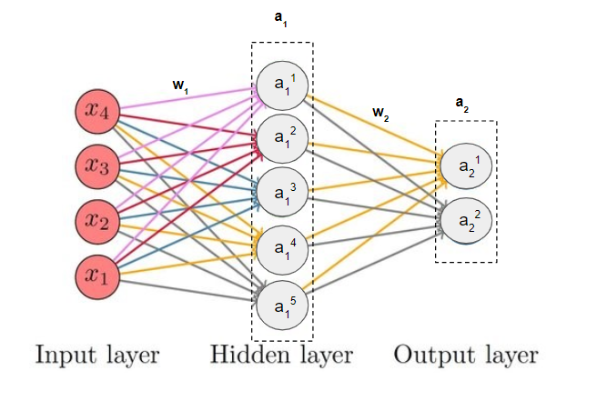
Note : All the terms w1, w2, a1, a2 (displayed in bold) are vectors. A vector has several elements within it, just as it is displayed for a1 and a2.
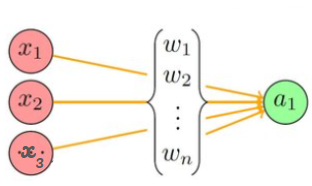
# Creating the Feedforward neural network
# 1 Input layer x.shape
# 1 hidden layer - 5 neurons - (1, 5)
# 1 output layer y.shape
def forward(x, w1, w2):
    # Hidden layer
    z1 = x.dot(w1)  # Input from layer 1
    a1 = sigmoid(z1)  # Output of layer 2

    # Output layer
    z2 = a1.dot(w2)  # Input of the output layer
    a2 = sigmoid(z2)  # Output of the output layer
    return a2
The forward function needs initial values of w1 and w2, to come up with first set of output in the first iteration. generate_wt function generates first few weights.
But why can’t we simply initialize with zeroes 0?
Initializing the neural network parameters, particularly the weights (w1 and w2), to all zeros leads to a significant issue known as the “symmetry problem”. When all weights are initialized to zero, hidden units within a layer become symmetric. This means they compute exactly the same function, making them indistinguishable.
That is why we initiate with random number. In practice, it is common to scale these random values by a small constant, such as 0.01.
# Initializing the weights randomly
def generate_wt(x, y):
    l = []
    for i in range(x * y):
        l.append(np.random.randn())
    return np.array(l).reshape(x, y)
Can you think of what would the NN look without even one hidden layer? Yes! Its would look something like a logistic regression.
Step 4— Loss Function
Building a NN is an iterative process, like any other traditional AI ML model. Each iteration predicts the output. The crucial question is whether the predicted output aligns to our expectation?
To measure the deviation of the predictions from the true values, we define our loss function. Here we take the mean square error (MSE) loss between the predicted output out and the true labels y.
# For loss, we will be using mean square error (MSE)
def loss(out, Y):
    s = (np.square(out - Y))
    s = np.sum(s) / len(y)
    return s
Step 5 — Backpropagation
Backpropagation is just a way of propagating the total loss back (*d2=*a2 — y) into the neural network to know how much of the loss every node is responsible for (w1_adj w2_adj). The backpropagation function back_prop calculates gradients and updates the weights w1 and w2 based on the error signals (d1 and d2) and the learning rate (alpha).
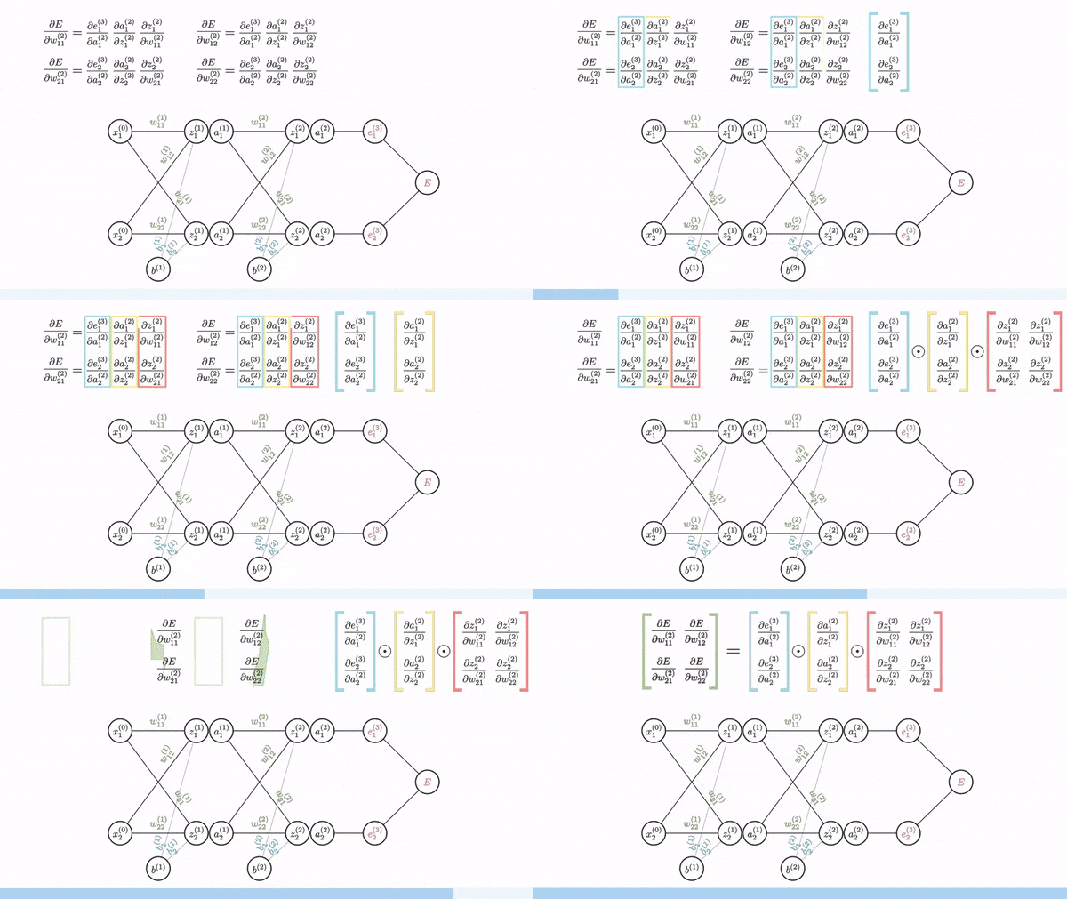
The sole purpose of backpropagation is to update the parameters/weights in the model. The weights are updated in a way that minimizes the loss by giving the nodes with higher error rates lower weights, and vice versa. Over time, after multiple repetition, the network becomes really good at the task because it has learned from its mistakes and fine-tuned its internal settings.
# Backpropagation of error
def back_prop(x, y, w1, w2, alpha):
    # Hidden layer Computation
    z1 = x.dot(w1)  # Weighted sum of input x
    a1 = sigmoid(z1)  # Output of layer 1 / input of layer 2

    # Output layer Computation
    z2 = a1.dot(w2)  # Input of the output layer
    a2 = sigmoid(z2)  # Output of the output layer

    # Error in the output layer
    d2 = (a2 - y) # a2 is output of NN , y is real output
    d1 = np.multiply(w2.dot(d2.transpose()).transpose(), np.multiply(a1, 1 - a1))

    # Gradient for w1 and w2
    w1_adj = x.transpose().dot(d1)
    w2_adj = a1.transpose().dot(d2)

    # Updating parameters/weights
    w1 = w1 - (alpha * w1_adj)
    w2 = w2 - (alpha * w2_adj)

    return w1, w2
Lets break d1 down in the ‘Error in the output layer ‘ segment of code
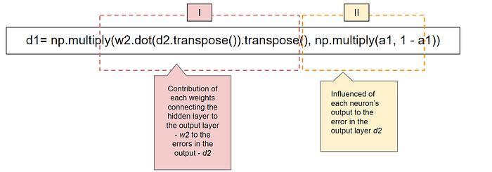
The first part (I) of the term d1 is matrix multiplication between w2 and d2. This tells us how much each weight in w2 contributed to the errors in the output.
The second part (II) is the derivative of a1. a1 represents the activation values of neurons. We have defined a sigmoid activation function and the derivative of the sigmoid function sigmoid(x) is sigmoid(x) * (1 — sigmoid(x)).
Step 6 — Training a Model
Now that we have defined all the main component of NN, we can call them to the train the neural network.
The train function iterates through a specified number of epochs and updates the weights using backpropagation. It also computes and prints the accuracy and loss during training.
def train(x, Y, w1, w2, alpha=0.01, epoch=10):
    # List to store accuracy and loss scores across epochs
    acc = []
    losss = []

    # Iterates over epoch
    for j in range(epoch):
        # List to store loss values for each training example in current epoch
        l = []


        # Within a epoch, iterates over each value of x
        for i in range(len(x)):
            out = forward(x[i], w1, w2) # Forward pass to compute output
            l.append(loss(out, Y[i])) # Calculating MSE loss for the current training example

            w1, w2 = back_prop(x[i], y[i], w1, w2, alpha) # Backpropagation and weight updates


        # Printing the accuracy at the current epoch
        print("epochs:", j + 1, "======== acc:", (1 - (sum(l) / len(x))) * 100)

        # Appending accuracy and loss values to the respective lists
        acc.append((1 - (sum(l) / len(x))) * 100)
        losss.append(sum(l) / len(x))
    return acc, losss, w1, w2
And that’s it!
With this you have already build a NN, your first NN.
Congrates, so proud of you!
In the part following this we will just create a predictive function which uses your model and gives you its predicted output and then we will test our model on a dummy data!
Step 7 — Predict/Output
The predict function takes input x as well as the trained weights from train function and makes prediction. It also displays an image and the predicted letter based on the highest output value.
def predict(x, w1, w2):
    Out = forward(x, w1, w2)
    return Out
Now it's ready to go!
Let's take some dummy data and get our first output.
# Creating data set

# A
a =[0, 0, 1, 1, 0, 1, 0, 1, 0, 0, 1, 0, 1, 1, 1, 1, 1, 1, 1, 0, 0, 0, 0, 1,
1, 0, 0, 0, 0, 1]
# B
b =[0, 1, 1, 1, 1, 0, 0, 1, 0, 0, 1, 0, 0, 1, 1, 1, 1, 0, 1, 1, 0, 0, 1, 0,
0, 1, 1, 1, 1, 0]
# C
c =[0, 1, 1, 1, 1, 0, 0, 1, 0, 0, 0, 0, 1, 1, 0, 0, 0, 0,0, 1, 0, 0, 0, 0,
0, 1, 1, 1, 1, 0]

# Creating labels
y =[[1, 0, 0],
[0, 1, 0],
[0, 0, 1]]

# converting data and labels into numpy array

x =[np.array(a).reshape(1, 30), np.array(b).reshape(1, 30),
                                np.array(c).reshape(1, 30)]


# Labels are also converted into NumPy array
y = np.array(y)

print(x, "\n\n", y)
Output >>
x = [array([[0, 0, 1, 1, 0, 1, 0, 1, 0, 0, 1, 0, 1, 1, 1, 1, 1, 1, 1, 0, 0, 0,
     0, 1, 1, 0, 0, 0, 0, 1]]),
     array([[0, 1, 1, 1, 1, 0, 0, 1, 0, 0, 1, 0, 0, 1, 1, 1, 1, 0, 1, 1, 0, 0,
     1, 0, 0, 1, 1, 1, 1, 0]]),
     array([[0, 1, 1, 1, 1, 0, 0, 1, 0, 0, 0, 0, 1, 1, 0, 0, 0, 0, 0, 1, 0, 0,
     0, 0, 0, 1, 1, 1, 1, 0]])]

 y = [[1 0 0]
 [0 1 0]
 [0 0 1]]
|Randomly generating out first weight,
Although thiw1 = generate_wt(30, 5)
w2 = generate_wt(5, 3)
Calling the train function and receiving the accuracy, loss and the final weights in acc, loss, w1, w2 respectively
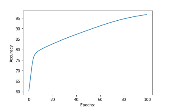
acc, loss, w1, w2 = train(x, y, w1, w2, 0.1, 100)
# plotting accuracy
plt.plot(acc)
plt.ylabel('Accuracy')
plt.xlabel("Epochs:")
plt.show()
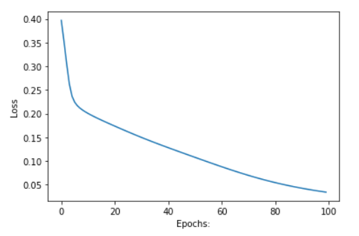
# plotting Loss
plt.plot(losss)
plt.ylabel('Loss')
plt.xlabel("Epochs:")
plt.show()
To get your final output, you can call the predict function. Do it yourself. I would love to hear your in the comment section! All the best!
#Your final output
predict(x, w1, w2)
This was a lengthy and simplified code. In reality to train a deep neural network, the amount to data that is required is simply huge. Python array aren’t that sophisticated. We have to replace it with tensors. Also we don’t code each and every function from scratch. Infact, we use torch.nn, it contains different classes that helps to build neural network models. All models in PyTorch inherit from the subclass nn.
Understanding Tensors in TensorFlow: The Building Blocks of Higher-Dimensional Data
TensorFlow, as the name suggests, revolves around the concept of tensors. Tensors serve as the fundamental building blocks upon which TensorFlow, one of the most powerful and widely-used deep learning frameworks, is built. But what exactly is a tensor, and how does it relate to the computations in TensorFlow? Let's try and understand the core concept of tensors, exploring their definition, properties with some examples.
What is a Tensor?
To begin with, let's demystify the term "tensor." At first glance, it might seem like a complex concept, but in reality, it's quite simple. In essence, a tensor is a generalization of a vector to higher dimensions. If you're familiar with linear algebra or basic vector calculus, you likely have encountered vectors before. Think of a vector as a data point; it doesn't necessarily have a fixed set of coordinates. For instance, in a two-dimensional space, a vector could consist of an (x, y) pair, while in a three-dimensional space, it might have three components (x, y, z). Tensors extend this idea further, allowing for an arbitrary number of dimensions.
According to the official TensorFlow documentation, a tensor is defined as follows:
A tensor is a generalization of vectors and matrices to potentially higher dimensions. Internally, TensorFlow represents tensors as n-dimensional arrays of base datatypes.
Let's break this down further. Tensors can hold numerical data, strings, or other datatypes, and they can have varying shapes and sizes. They serve as the primary objects for storing and manipulating data within TensorFlow.
Creating Tensors
Now that we have a basic understanding of tensors, let's see how we can create them in TensorFlow. Below are some examples of creating tensors using TensorFlow's API:
import tensorflow as tf

# Creating a string tensor
string_tensor = tf.Variable("Hello, TensorFlow!", tf.string)

# Creating a number tensor
number_tensor = tf.Variable(123, tf.int16)

# Creating a floating-point tensor
float_tensor = tf.Variable(3.14, tf.float32)
In the above code snippets, we use TensorFlow's tf.Variable function to create tensors of different datatypes. Each tensor has an associated datatype (tf.string, tf.int16, tf.float32) and an initial value. These tensors represent scalar values since they contain only one element.
Rank of Tensors
The rank, also known as the degree, of a tensor refers to the number of dimensions it possesses. Let's explore the concept of rank with some examples:
Rank 0 Tensor (Scalar): This tensor represents a single value without any dimensions.
Rank 1 Tensor (Vector): It consists of a one-dimensional array of values.
Rank 2 Tensor (Matrix): This tensor contains a two-dimensional array of values.
Higher Rank Tensors: Tensors with more than two dimensions follow the same pattern.
Here's how we determine the rank of a tensor using TensorFlow's tf.rank method:
# Determining the rank of a tensor
print("Rank of string_tensor:", tf.rank(string_tensor).numpy())
print("Rank of number_tensor:", tf.rank(number_tensor).numpy())
print("Rank of float_tensor:", tf.rank(float_tensor).numpy())
In the above code, tf.rank(tensor) returns the rank of the tensor. The .numpy() method is used to extract the rank value as a NumPy array.
Shape of Tensors
At its core, a tensor is a multidimensional array that can hold data of varying dimensions and sizes. Tensor shapes play a pivotal role in defining the structure and dimensions of these arrays. The shape of a tensor describes the number of elements along each dimension. It provides crucial information about the structure of the tensor. Let's illustrate this concept with examples:
For a rank 0 tensor (scalar), the shape is empty since it has no dimensions.
For a rank 1 tensor (vector), the shape corresponds to the length of the array.
For a rank 2 tensor (matrix), the shape represents the number of rows and columns.
Let's see this with example
import tensorflow as tf

# Tensor with Rank 0 (Scalar)
tensor_rank_0 = tf.constant(42)
print("Tensor with Rank 0 (Scalar):")
print("Tensor:", tensor_rank_0)
print("Shape:", tensor_rank_0.shape)
print("Value:", tensor_rank_0.numpy())
print()

# Tensor with Rank 1 (Vector)
tensor_rank_1 = tf.constant([1, 2, 3, 4, 5])
print("Tensor with Rank 1 (Vector):")
print("Tensor:", tensor_rank_1)
print("Shape:", tensor_rank_1.shape)
print("Values:", tensor_rank_1.numpy())
print()

# Tensor with Rank 2 (Matrix)
tensor_rank_2 = tf.constant([[1, 2, 3], [4, 5, 6], [7, 8, 9]])
print("Tensor with Rank 2 (Matrix):")
print("Tensor:", tensor_rank_2)
print("Shape:", tensor_rank_2.shape)
print("Values:")
print(tensor_rank_2.numpy())
Output
Ou
Tensor with Rank 0 (Scalar):
Tensor: tf.Tensor(42, shape=(), dtype=int32)
Shape: ()
Value: 42

Tensor with Rank 1 (Vector):
Tensor: tf.Tensor([1 2 3 4 5], shape=(5,), dtype=int32)
Shape: (5,)
Values: [1 2 3 4 5]

Tensor with Rank 2 (Matrix):
Tensor: tf.Tensor(
[[1 2 3]
 [4 5 6]
 [7 8 9]], shape=(3, 3), dtype=int32)
Shape: (3, 3)
Values:
[[1 2 3]
 [4 5 6]
 [7 8 9]]
In these examples:
tensor_rank_0is a scalar tensor with rank 0 and no dimensions.tensor_rank_1is a vector tensor with rank 1 and a shape of(5,).tensor_rank_2is a matrix tensor with rank 2 and a shape of(3, 3).
Tensor Manipulation
Tensor manipulation forms the backbone of many TensorFlow operations, enabling us to reshape, transpose, concatenate, and manipulate tensors in various ways. Understanding tensor manipulation techniques is crucial for data preprocessing, model building, and optimization. Let's delve into some key tensor manipulation operations:
Reshaping Tensors
Reshaping tensors allows us to change their dimensions, rearrange their shape, and adapt them to different requirements. Whether it's converting between 1D, 2D, or higher-dimensional arrays, reshaping is a fundamental operation in data preprocessing and model preparation.
import tensorflow as tf

# Create a tensor
tensor = tf.constant([[1, 2, 3], [4, 5, 6]])

# Reshape the tensor
reshaped_tensor = tf.reshape(tensor, [3, 2])

print("Original Tensor:")
print(tensor.numpy())
print("Reshaped Tensor:")
print(reshaped_tensor.numpy())
output
Original Tensor:
[[1 2 3]
 [4 5 6]]
Reshaped Tensor:
[[1 2]
 [3 4]
 [5 6]]
Slicing Tensors
Slicing operations allow us to extract specific subsets of data from tensors along one or more dimensions. By specifying the start and end indices, we can extract desired portions of the data for further processing.
# Slice the tensor
sliced_tensor = tensor[:, 1:]

print("Original Tensor:")
print(tensor.numpy())
print("Sliced Tensor:")
print(sliced_tensor.numpy())
output
Original Tensor:
[[1 2 3]
 [4 5 6]]
Sliced Tensor:
[[2 3]
 [5 6]]
Concatenating Tensors
Concatenating tensors involves combining multiple tensors along specified dimensions. This operation is useful for merging datasets, assembling model inputs, and creating batches of data.
# Create tensors for concatenation
tensor_a = tf.constant([[1, 2], [3, 4]])
tensor_b = tf.constant([[5, 6], [7, 8]])

# Concatenate tensors along axis 0
concatenated_tensor = tf.concat([tensor_a, tensor_b], axis=0)

print("Tensor A:")
print(tensor_a.numpy())
print("Tensor B:")
print(tensor_b.numpy())
print("Concatenated Tensor:")
print(concatenated_tensor.numpy())
output
Tensor A:
[[1 2]
 [3 4]]
Tensor B:
[[5 6]
 [7 8]]
Concatenated Tensor:
[[1 2]
 [3 4]
 [5 6]
 [7 8]]
Broadcasting
Broadcasting is a powerful technique that enables element-wise operations between tensors of different shapes. TensorFlow automatically aligns dimensions and extends smaller tensors to match the shape of larger ones, simplifying mathematical operations and improving computational efficiency.
# Perform broadcasting operation
tensor_a = tf.constant([[1, 2], [3, 4]])
tensor_b = tf.constant([5, 6])

result = tensor_a + tensor_b

print("Tensor A:")
print(tensor_a.numpy())
print("Tensor B:")
print(tensor_b.numpy())
print("Result after Broadcasting:")
print(result.numpy())
output
Tensor A:
[[1 2]
 [3 4]]
Tensor B:
[5 6]
Result after Broadcasting:
[[ 6  8]
 [ 8 10]]
Transposing Tensors
Tensor transposition involves swapping the dimensions of a tensor, thereby altering its orientation. Transposing tensors is particularly useful for tasks such as matrix multiplication, convolution operations, and feature extraction.
import tensorflow as tf

# Create a tensor
tensor = tf.constant([[1, 2, 3], [4, 5, 6]])

# Transpose the tensor
transposed_tensor = tf.transpose(tensor)

print("Original Tensor:")
print(tensor.numpy())
print("Transposed Tensor:")
print(transposed_tensor.numpy())
output
Original Tensor:
[[1 2 3]
 [4 5 6]]
Transposed Tensor:
[[1 4]
 [2 5]
 [3 6]]
Applications of Tensors in Machine Learning
Deep Learning: Deep neural networks rely heavily on tensors to store and manipulate data. Tensors represent inputs, weights, biases, and gradients throughout the training process, enabling deep learning models to handle complex tasks such as image classification, speech recognition, and natural language understanding.
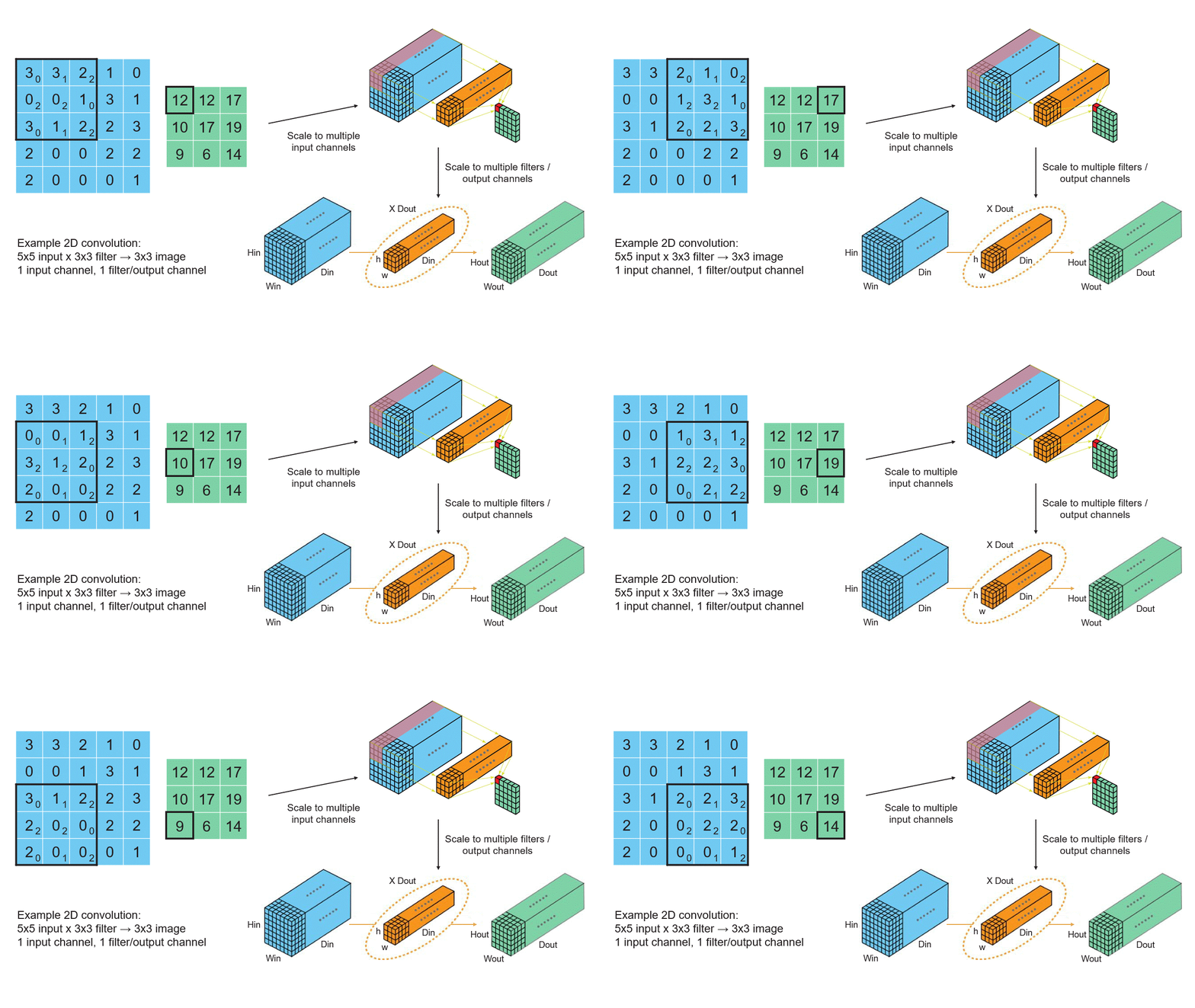
Convolutional Neural Networks (CNNs): CNNs, widely used in computer vision tasks, use tensor-based convolution operations to extract features from images and learn hierarchical representations. These operations involve applying filters (kernels) to multidimensional input data.
Recurrent Neural Networks (RNNs): RNNs, commonly used for sequential data, process input sequences as tensors over time, making them suitable for tasks like language modeling, speech recognition, and stock market prediction.
Tensor Factorization: Tensor factorization techniques, like Tucker decomposition or CP decomposition, are used in recommendation systems and collaborative filtering to model user-item interactions more efficiently. These methods help identify latent factors and improve the recommendation accuracy.
Code
Here’s a complete Python code example using the NumPy library to work with tensors and then visualize them with a plot using the Matplotlib library. This example will create a 2D tensor, perform some basic tensor operations, and then plot the tensor as an image.
mport numpy as np
import matplotlib.pyplot as plt

# Create a 2D tensor (matrix)
tensor = np.array([[1, 2, 3],
                   [4, 5, 6],
                   [7, 8, 9]])

# Print the tensor
print("Tensor:")
print(tensor)

# Perform some tensor operations
tensor_sum = np.sum(tensor)
tensor_mean = np.mean(tensor)
tensor_transpose = np.transpose(tensor)

# Print the results of tensor operations
print("\nSum of the tensor elements:", tensor_sum)
print("Mean of the tensor elements:", tensor_mean)
print("\nTranspose of the tensor:")
print(tensor_transpose)

# Visualize the tensor as an image using Matplotlib
plt.imshow(tensor, cmap='viridis', interpolation='nearest')
plt.title("2D Tensor Visualization")
plt.colorbar(label="Value")
plt.show()
output
Tensor:
[[1 2 3]
 [4 5 6]
 [7 8 9]]

Sum of the tensor elements: 45
Mean of the tensor elements: 5.0

Transpose of the tensor:
[[1 4 7]
 [2 5 8]
 [3 6 9]]
This code creates a simple 3x3 2D tensor, performs basic operations (sum, mean, and transpose), and then visualizes the tensor as an image using Matplotlib with a color bar.
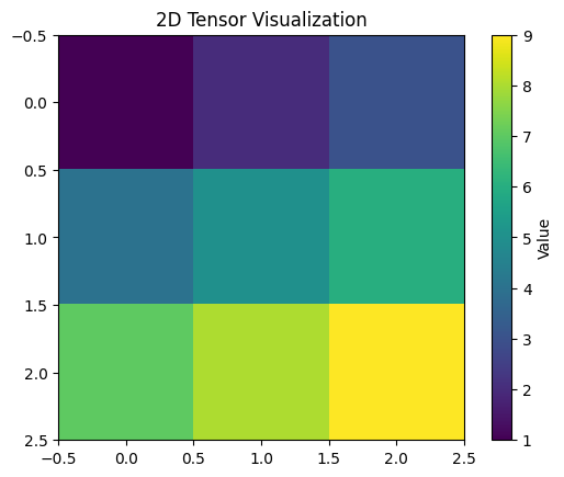
You can run this code in a Python environment, and it will display the tensor as an image using Matplotlib’s imshow function. Adjust the tensor values or operations as needed for your specific use case.
PyTorch for building neural networks
PyTorch is an open source deep learning library based on Torch. It provides a flexible neural networks library and automatic differentiation capabilities. Here is a simple example of a neural network in PyTorch:
# Imports
import torch
import torch.nn as nn

# Model architecture
model = nn.Sequential(
  nn.Linear(in_features=input_size, out_features=hidden_size),
  nn.ReLU(),
  nn.Linear(in_features=hidden_size, out_features=output_size),
)

# Forward pass
outputs = model(inputs)

# Loss calculation
loss = loss_fn(outputs, targets)

# Backpropagation
loss.backward()

# Update weights
optimizer.step()
The key aspects are:
nn.Modulecontains layers andforward()defines the forward pass.nn.functionalprovides common functions like activation, loss etc.torch.optimoptimizers like SGD, Adam update weights.backward()auto calculates gradients.
TensorFlow for building neural networks
TensorFlow is another popular open source library for high performance numerical computation and deep learning. Here is an example of building a dense neural network in TensorFlow:
# Imports and input data

import tensorflow as tf
inputs = tf.keras.Input(shape=(input_size,))

# Dense layers
x = tf.keras.layers.Dense(hidden_size, activation='relu')(inputs)
outputs = tf.keras.layers.Dense(output_size, activation='sigmoid')(x)

# Model and compilation
model = tf.keras.Model(inputs=inputs, outputs=outputs)
model.compile(optimizer='adam',
              loss=tf.keras.losses.BinaryCrossentropy(),
              metrics=['accuracy'])

# Train the model
model.fit(data, targets, epochs=10)
Keras high-level API for building neural networks
Keras is a high-level API that can use TensorFlow, PyTorch or other backends. It makes building neural networks even more convenient. Here is an example:
# Imports and data

from tensorflow import keras
from keras.layers import Dense

inputs = keras.Input(shape=(input_size,))

# Layers
x = Dense(hidden_size, activation='relu')(inputs)
outputs = Dense(output_size, activation='sigmoid')(x)

# Model
model = keras.Model(inputs=inputs, outputs=outputs)

# Compile and train
model.compile(optimizer='adam', loss='binary_crossentropy')
model.fit(data, targets, epochs=10)
The simplicity of the Keras API makes it easy to build models quickly.
To summarize, PyTorch provides flexibility, TensorFlow enables high performance, and Keras offers convenience. All three are great choices for building and training neural networks in Python.
What are Neural Networks?
Neural Networks are a class of models within the general machine learning literature. So for example, if you took a Coursera course on machine learning, neural networks will likely be covered. Neural networks are a specific set of algorithms that has revolutionized the field of machine learning. They are inspired by biological neural networks and the current so called deep neural networks have proven to work quite very well. Neural Networks are themselves general function approximations, that is why they can be applied to literally almost any machine learning problem where the problem is about learning a complex mapping from the input to the output space.
Here are the 3 reasons to convince you to study neural computation:
To understand how the brain actually works: It’s very big and very complicated and made of stuff that dies when you poke it around. So we need to use computer simulations.
To understand a style of parallel computation inspired by neurons and their adaptive connections: It’s a very different style from sequential computation.
To solve practical problems by using novel learning algorithms inspired by the brain: Learning algorithms can be very useful even if they are not how the brain actually works.
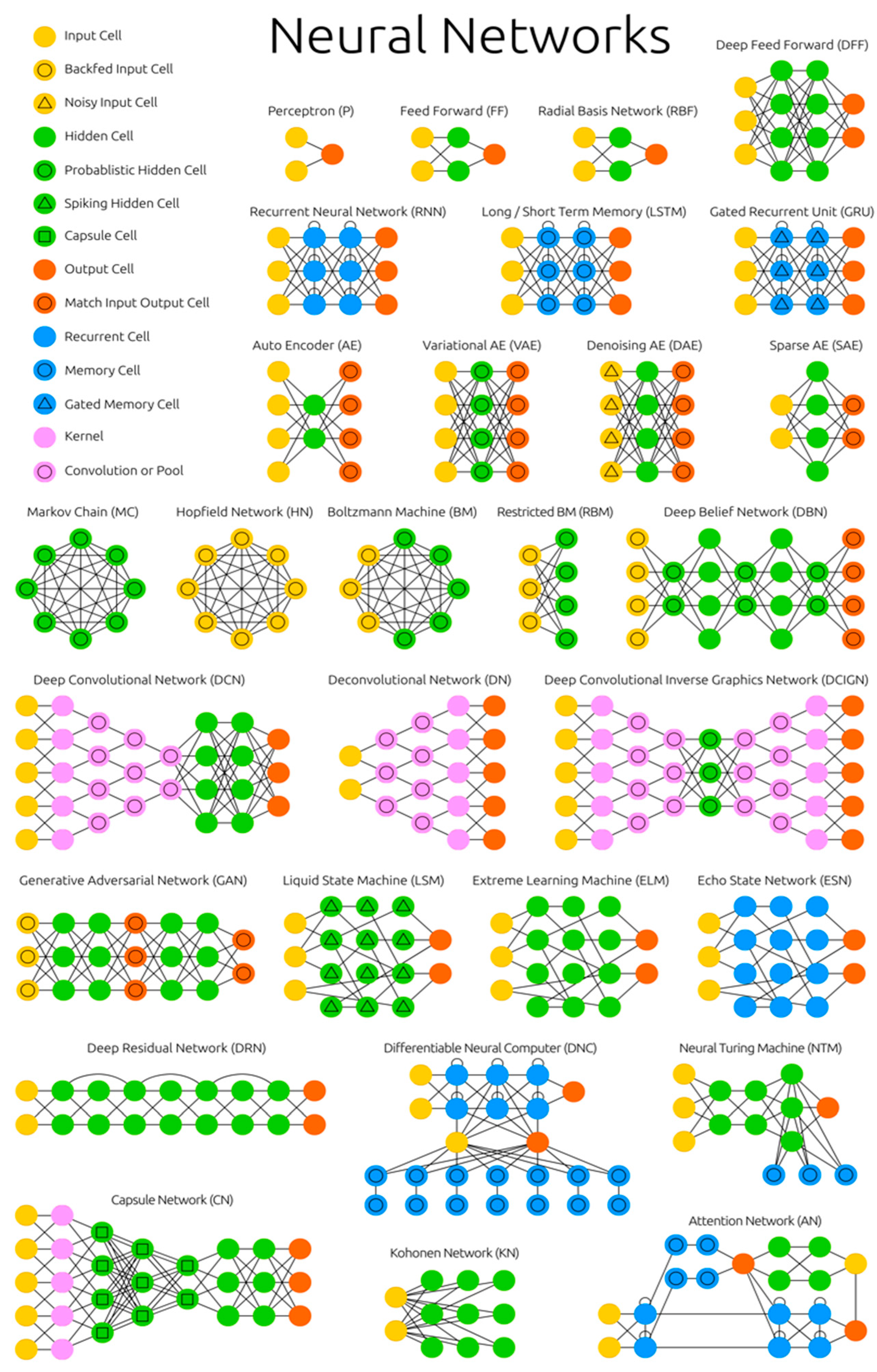
Top 10 Neural Network Architectures You Need to Know
1 — Perceptrons
Considered the first generation of neural networks, Perceptrons are simply computational models of a single neuron. Perceptron was originally coined by Frank Rosenblatt in his paper, “The perceptron: a probabilistic model for information storage and organization in the brain” (1956) . Also called feed-forward neural network, perceptron feeds information from the front to the back. Training perceptrons usually requires back-propagation, giving the network paired datasets of inputs and outputs. Inputs are sent into the neuron, processed, and result in an output. The error being back propagated is often some variation of the difference between the input and the output. Given that the network has enough hidden neurons, it can theoretically always model the relationship between the input and output. Practically their use is a lot more limited but they are popularly combined with other networks to form new networks.
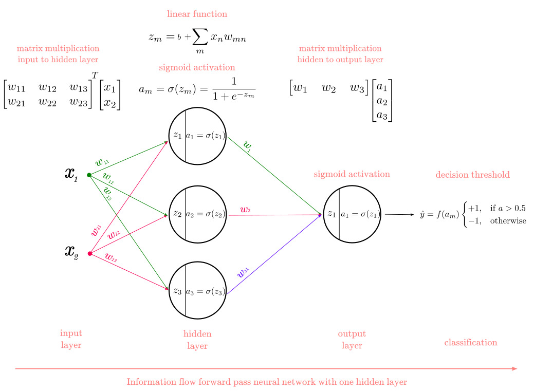
However, Perceptrons do have limitations: If you choose features by hand and you have enough features, you can do almost anything. For binary input vectors, we can have a separate feature unit for each of the exponentially many binary vectors and so we can make any possible discrimination on binary input vectors. But once the hand-coded features have been determined, there are very strong limitations on what a perceptron can learn.
2 — Convolutional Neural Networks
In 1998, Yann LeCun and his collaborators developed a really good recognizer for handwritten digits called LeNet. It used back propagation in a feedforward net with many hidden layers, many maps of replicated units in each layer, pooling of the outputs of nearby replicated units, a wide net that can cope with several characters at once even if they overlap, and a clever way of training a complete system, not just a recognizer. Later it is formalized under the name convolutional neural networks (CNNs).
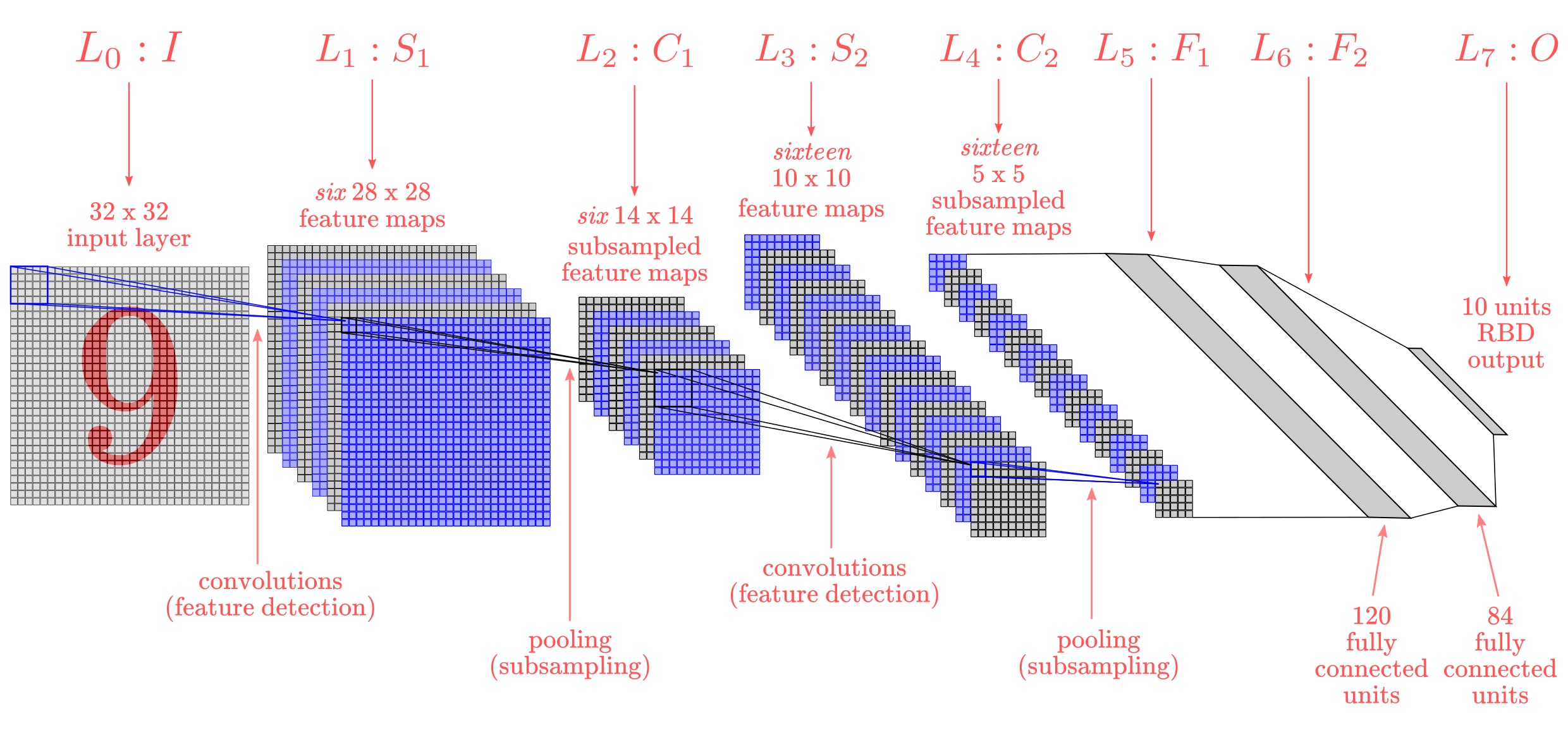
Convolutional Neural Networks are quite different from most other networks. They are primarily used for image processing but can also be used for other types of input such as as audio. A typical use case for CNNs is where you feed the network images and the network classifies the data. CNNs tend to start with an input “scanner” which is not intended to parse all the training data at once. For example, to input an image of 100 x 100 pixels, you wouldn’t want a layer with 10 000 nodes. Rather, you create a scanning input layer of say 10 x 10 which you feed the first 10 x 10 pixels of the image. Once you passed that input, you feed it the next 10 x 10 pixels by moving the scanner one pixel to the right.
his input data is then fed through convolutional layers instead of normal layers, where not all nodes are connected to all nodes. Each node only concerns itself with close neighboring cells. These convolutional layers also tend to shrink as they become deeper, mostly by easily divisible factors of the input. Besides these convolutional layers, they also often feature pooling layers. Pooling is a way to filter out details: a commonly found pooling technique is max pooling, where we take say 2 x 2 pixels and pass on the pixel with the most amount of red. If you want to dig deeper into CNNs, read Yann LeCun’s original paper — “Gradient-based learning applied to document recognition” (1998).
3 — Recurrent Neural Networks
To understand RNNs, we need to have a brief overview on sequence modeling. When applying machine learning to sequences, we often want to turn an input sequence into an output sequence that lives in a different domain; for example, turn a sequence of sound pressures into a sequence of word identities. When there is no separate target sequence, we can get a teaching signal by trying to predict the next term in the input sequence. The target output sequence is the input sequence with an advance of 1 step. This seems much more natural than trying to predict one pixel in an image from the other pixels, or one patch of an image from the rest of the image. Predicting the next term in a sequence blurs the distinction between supervised and unsupervised learning. It uses methods designed for supervised learning, but it doesn’t require a separate teaching signal.
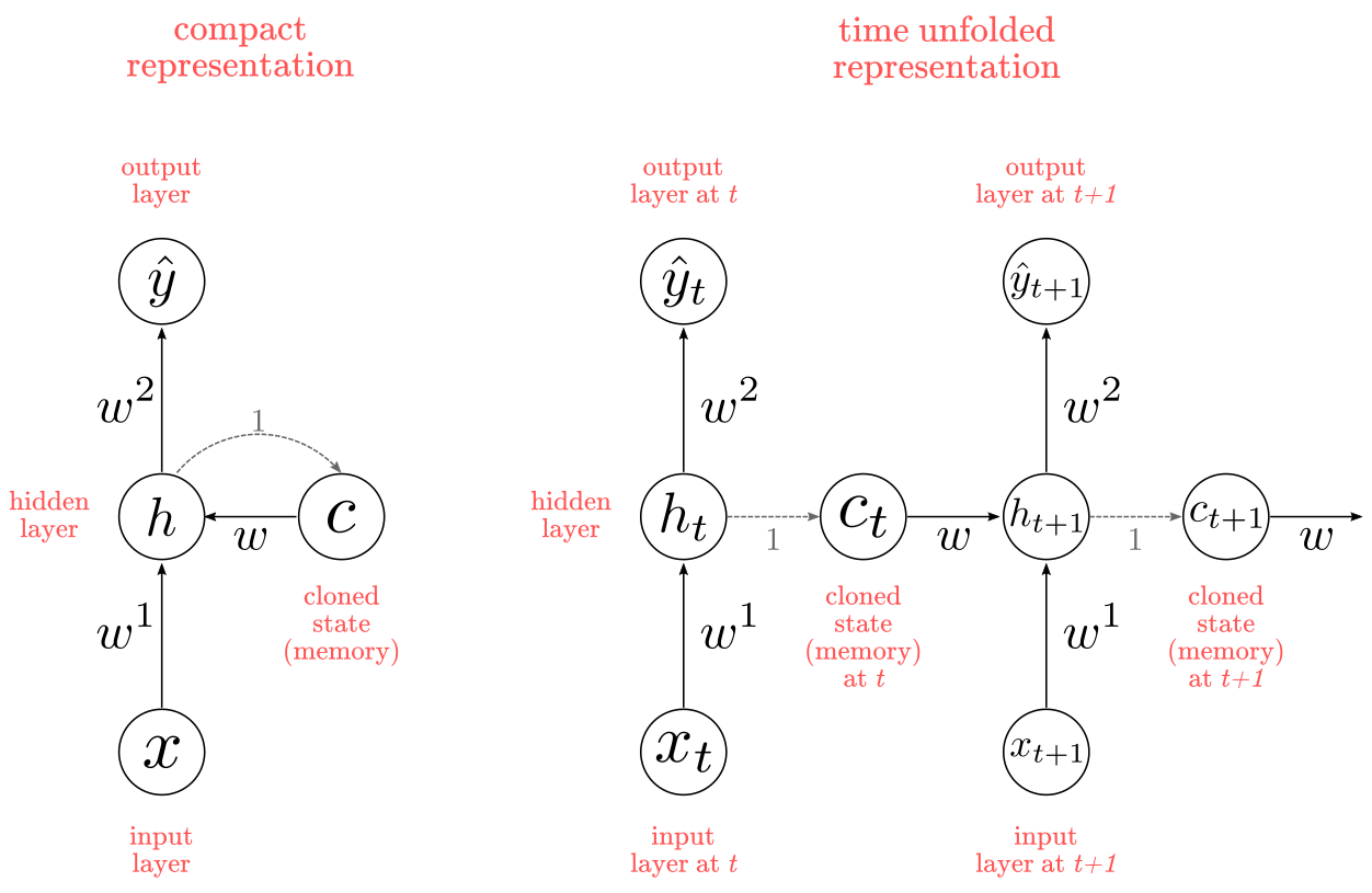
Memoryless models are the standard approach to this task. In particular, autoregressive models can predict the next term in a sequence from a fixed number of previous terms using “delay taps; and feed-forwad neural nets are generalized autoregressive models that use one or more layers of non-linear hidden units. However, if we give our generative model some hidden state, and if we give this hidden state its own internal dynamics, we get a much more interesting kind of model: It can store information in its hidden state for a long time. If the dynamics is noisy and the way it generates outputs from its hidden state is noisy, we can never know its exact hidden state. The best we can do is to infer a probability distribution over the space of hidden state vectors. This inference is only tractable for 2 types of hidden state model.
Originally introduced in Jeffrey Elman’s “Finding structure in time” (1990) , recurrent neural networks (RNNs) are basically perceptrons; however, unlike perceptrons which are stateless, they have connections between passes, connections through time. RNNs are very powerful, because they combine 2 properties: 1) distributed hidden state that allows them to store a lot of information about the past efficiently; and 2) non-linear dynamics that allows them to update their hidden state in complicated ways. With enough neurons and time, RNNs can compute anything that can be computed by your computer. So what kinds of behavior can RNNs exhibit? They can oscillate, they can settle to point attractors, they can behave chaotically. And they could potentially learn to implement lots of small programs that each capture a nugget of knowledge and run in parallel, interacting to produce very complicated effects.
One big problem with RNNs is the vanishing (or exploding) gradient problem where, depending on the activation functions used, information rapidly gets lost over time. Intuitively this wouldn’t be much of a problem because these are just weights and not neuron states, but the weights through time is actually where the information from the past is stored; if the weight reaches a value of 0 or 1 000 000, the previous state won’t be very informative. RNNs can in principle be used in many fields as most forms of data that don’t actually have a timeline (i.e. unlike sound or video) can be represented as a sequence. A picture or a string of text can be fed one pixel or character at a time, so the time dependent weights are used for what came before in the sequence, not actually from what happened x seconds before. In general, recurrent networks are a good choice for advancing or completing information, such as autocompletion.
4 — Long / Short Term Memory
Hochreiter & Schmidhuber (1997) solved the problem of getting a RNN to remember things for a long time by building what known as long-short term memory networks (LSTMs). LSTMs networks try to combat the vanishing / exploding gradient problem by introducing gates and an explicitly defined memory cell. The memory cell stores the previous values and holds onto it unless a “forget gate” tells the cell to forget those values. LSTMs also have a “input gate” which adds new stuff to the cell and an “output gate” which decides when to pass along the vectors from the cell to the next hidden state.
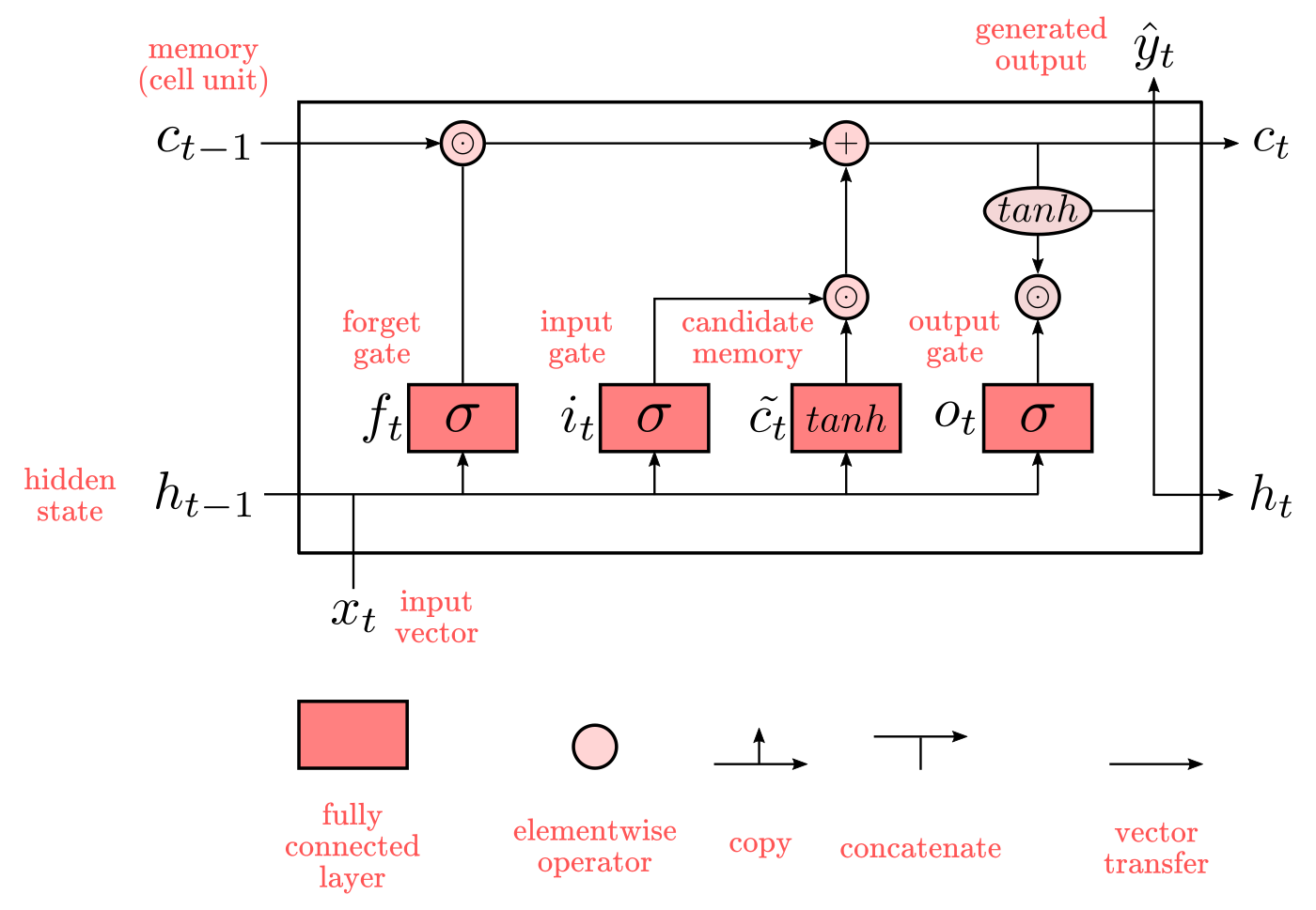
Recall that with all RNNs, the values coming in from X_train and H_previous are used to determine what happens in the current hidden state. And the results of the current hidden state (H_current) are used to determine what happens in the next hidden state. LSTMs simply add a cell layer to make sure the transfer of hidden state information from one iteration to the next is reasonably high. Put another way, we want to remember stuff from previous iterations for as long as needed, and the cells in LSTMs allow this to happen. LSTMs have been shown to be able to learn complex sequences, such as writing like Shakespeare or composing primitive music.
5 — Gated Recurrent Unit
Gated recurrent units (GRUs) are a slight variation on LSTMs. They take X_train and H_previous as inputs. They perform some calculations and then pass along H_current. In the next iteration X_train.next and H_current are used for more calculations, and so on. What makes them different from LSTMs is that GRUs don’t need the cell layer to pass values along. The calculations within each iteration insure that the H_current values being passed along either retain a high amount of old information or are jump-started with a high amount of new information.
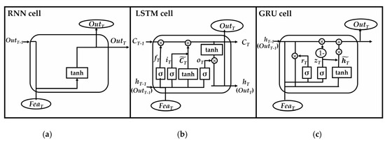
In most cases, GRUs function very similarly to LSTMs, with the biggest difference being that GRUs are slightly faster and easier to run (but also slightly less expressive). In practice these tend to cancel each other out, as you need a bigger network to regain some expressiveness which then in turn cancels out the performance benefits. In some cases where the extra expressiveness is not needed, GRUs can outperform LSTMs. You can read more about GRU from Junyoung Chung’s 2014 paper “Empirical evaluation of gated recurrent neural networks on sequence modeling”
6 — Hopfield Network
Recurrent networks of non-linear units are generally very hard to analyze. They can behave in many different ways: settle to a stable state, oscillate, or follow chaotic trajectories that cannot be predicted far into the future. To resolve this problem, John Hopfield introduced Hopfield Net in his 1982 paper “Neural networks and physical systems with emergent collective computational abilities” . A Hopfield network (HN) is a network where every neuron is connected to every other neuron; it is a completely entangled plate of spaghetti as even all the nodes function as everything. Each node is input before training, then hidden during training and output afterwards. The networks are trained by setting the value of the neurons to the desired pattern after which the weights can be computed. The weights do not change after this. Once trained for one or more patterns, the network will always converge to one of the learned patterns because the network is only stable in those states.
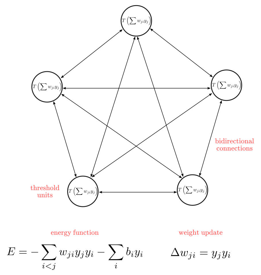
There is another computational role for Hopfield nets. Instead of using the net to store memories, we use it to construct interpretations of sensory input. The input is represented by the visible units, the interpretation is represented by the states of the hidden units, and the badness of the interpretation is represented by the energy.
Unfortunately people shown that Hopfield net is very limited in its capacity. A Hopfield net of N units can only memorize 0.15N patterns because of the so-called spurious minima in its energy function. The idea is that since the energy function is continuous in the space of its weights, if two local minima are too close, they might “fall” into each other to create a single local minima which doesn’t correspond to any training sample, while forgetting about the two samples it is supposed to memorize. This phenomenon significantly limits the number of samples that a Hopfield net can learn.
— Boltzmann Machine
A Boltzmann Machine is a type of stochastic recurrent neural network. It can be seen as the stochastic, generative counterpart of Hopfield nets. It was one of the first neural networks capable of learning internal representations, and is able to represent and solve difficult combinatoric problems. First introduced by Geoffrey Hinton and Terrence Sejnowski in “Learning and relearning in Boltzmann machines” (1986), Boltzmann machines are a lot like Hopfield Networks, but some neurons are marked as input neurons and others remain “hidden”. The input neurons become output neurons at the end of a full network update. It starts with random weights and learns through back-propagation. Compared to a Hopfield Net, the neurons mostly have binary activation patterns.
The goal of learning for Boltzmann machine learning algorithm is to maximize the product of the probabilities that the Boltzmann machine assigns to the binary vectors in the training set. This is equivalent to maximizing the sum of the log probabilities that the Boltzmann machine assigns to the training vectors. It is also equivalent to maximizing the probability that we would obtain exactly the N training cases if we did the following: 1) Let the network settle to its stationary distribution N different time with no external input; and 2) Sample the visible vector once each time. An efficient mini-batch learning procedure was proposed for Boltzmann Machines by Salakhutdinov and Hinton in 2012.
For the positive phase, first initialize the hidden probabilities at 0.5, then clamp a data vector on the visible units, then update all the hidden units in parallel until convergence using mean field updates. After the net has converged, record PiPj for every connected pair of units and average this over all data in the mini-batch.
For the negative phase: first keep a set of “fantasy particles.” Each particle has a value that is a global configuration. Then sequentially update all the units in each fantasy particle a few times. For every connected pair of units, average SiSj over all the fantasy particles.
In a general Boltzmann machine, the stochastic updates of units need to be sequential. There is a special architecture that allows alternating parallel updates which are much more efficient (no connections within a layer, no skip-layer connections). This mini-batch procedure makes the updates of the Boltzmann machine more parallel. This is called a Deep Boltzmann Machine (DBM), a general Boltzmann machine with a lot of missing connections.

8 — Deep Belief Networks
Back-propagation is considered the standard method in artificial neural networks to calculate the error contribution of each neuron after a batch of data is processed. However, there are some major problems using back-propagation. Firstly, it requires labeled training data; while almost all data is unlabeled. Secondly, the learning time does not scale well, which means it is very slow in networks with multiple hidden layers. Thirdly, it can get stuck in poor local optima, so for deep nets they are far from optimal.
To overcome the limitations of back-propagation, researchers have considered using unsupervised learning approaches. This helps keep the efficiency and simplicity of using a gradient method for adjusting the weights, but also use it for modeling the structure of the sensory input. In particular, they adjust the weights to maximize the probability that a generative model would have generated the sensory input. The question is what kind of generative model should we learn? Can it be an energy-based model like a Boltzmann machine? Or a causal model made of idealized neurons? Or a hybrid of the two?

Yoshua Bengio came up with Deep Belief Networks in his 2007 paper “Greedy layer-wise training of deep networks”, which have been shown to be effectively trainable stack by stack. This technique is also known as greedy training, where greedy means making locally optimal solutions to get to a decent but possibly not optimal answer. A belief net is a directed acyclic graph composed of stochastic variables. Using belief net, we get to observe some of the variables and we would like to solve 2 problems: 1) The inference problem: Infer the states of the unobserved variables, and 2) The learning problem: Adjust the interactions between variables to make the network more likely to generate the training data.
Deep Belief Networks can be trained through contrastive divergence or back-propagation and learn to represent the data as a probabilistic model. Once trained or converged to a stable state through unsupervised learning, the model can be used to generate new data. If trained with contrastive divergence, it can even classify existing data because the neurons have been taught to look for different features.
9 — Autoencoders
Autoencoders are neural networks designed for unsupervised learning, i.e. when the data is not labeled. As a data-compression model, they can be used to encode a given input into a representation of smaller dimension. A decoder can then be used to reconstruct the input back from the encoded version.
The work they do is very similar to Principal Component Analysis, which is generally used to represent a given input using less number of dimensions than originally present. So for example, in NLP if you represent a word as a vector of 100 numbers, you could use PCA to represent it in 10 numbers. Of course, that would result in loss of some information, but it is a good way to represent your input if you can only work with a limited number of dimensions. Also, it is a good way to visualize the data because you can easily plot the reduced dimensions on a 2D graph, as opposed to a 100-dimensional vector. Autoencoders do similar work — the difference being that they can use non-linear transformations to encode the given vector into smaller dimensions (as compared to PCA which is a linear transformation). So it can generate more complex encodings.
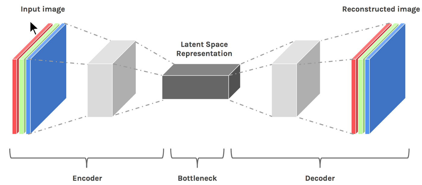
They can be used for dimension reduction, pretraining of other neural networks, for data generation etc. There are a couple of reasons: (1) They provide flexible mappings both ways, (2) the learning time is linear (or better) in the number of training cases, and (3) the final encoding model is fairly compact and fast. However, it turned out to be very difficult to optimize deep auto encoders using back propagation. With small initial weights, the back propagated gradient dies. Nowadays they are rarely used in practical applications, mostly because in key areas for which they where once considered to be a breakthrough (such as layer-wise pre-training), it turned out that vanilla supervised learning works better. Check out the original paper by Bourlard and Kamp dated back in 1988 .
10 — Generative Adversarial Network
In “Generative adversarial nets” (2014), Ian Goodfellow introduced a new breed of neural network, in which 2 networks work together. Generative Adversarial Networks (GANs) consist of any two networks (although often a combination of Feed Forwards and Convolutional Neural Nets), with one tasked to generate content (generative) and the other has to judge content (discriminative). The discriminative model has the task of determining whether a given image looks natural (an image from the dataset) or looks like it has been artificially created. The task of the generator is to create natural looking images that are similar to the original data distribution. This can be thought of as a zero-sum or minimax two player game. The analogy used in the paper is that the generative model is like “a team of counterfeiters, trying to produce and use fake currency” while the discriminative model is like “the police, trying to detect the counterfeit currency”. The generator is trying to fool the discriminator while the discriminator is trying to not get fooled by the generator. As the models train through alternating optimization, both methods are improved until a point where the “counterfeits are indistinguishable from the genuine articles”.

According to Yann LeCun, these networks could be the next big development. They are one of the few successful techniques in unsupervised machine learning, and are quickly revolutionizing our ability to perform generative tasks. Over the last few years, we’ve come across some very impressive results. There is a lot of active research in the field to apply GANs for language tasks, to improve their stability and ease of training, and so on.
They are already being applied in industry for a variety of applications ranging from interactive image editing, 3D shape estimation, drug discovery, semi-supervised learning to robotics.
Neural Network from scratch
This isn’t one of those articles where you’ll be given an overview of the structure of a neural net. Neither is this a “for dummies” article where you’ll be taught how to use sklearn and scipy. Instead, this is more of a walk-through, where I provide all the necessary code to build a neural net from scratch, using no libraries whatsoever (well, except numpy and some visualisation related libraries, and sklearn.datasets to get a dataset), as well as information for everything to make sense. Firstly, it’s important for you to read one of those “Introduction” articles before reading this, because this isn’t a topic I can cover in a post of rational length.
Automatic differentiation
The reason that gradient descent works so smoothly for incredibly complicated functions, with even more complicated gradients (as functions) is because, just like most problems, we can break big problems into smaller ones. This is done by the automatic differentiation, which is basically a clever way of using the multi-variable chain rule, which is given by :
An important application of computational graphs is automatic differentiation (AD). In general, there are three modes of AD: reverse-mode, forward-mode, and mixed mode. In this tutorial, we focus on the forward-mode and reverse-mode.
Basically, the forward mode and the reverse mode automatic differenation both use the. chain rule for computing the gradients. They evaluate the gradients of "small" functions analytically (symbolically) and chain all the computed numerical gradients via the chain rule
$$\frac{\partial f\circ g (x)}{\partial x} = \frac{\partial f'\circ g(x)}{\partial g} {\frac{\partial g'(x)}{\partial x}}$$
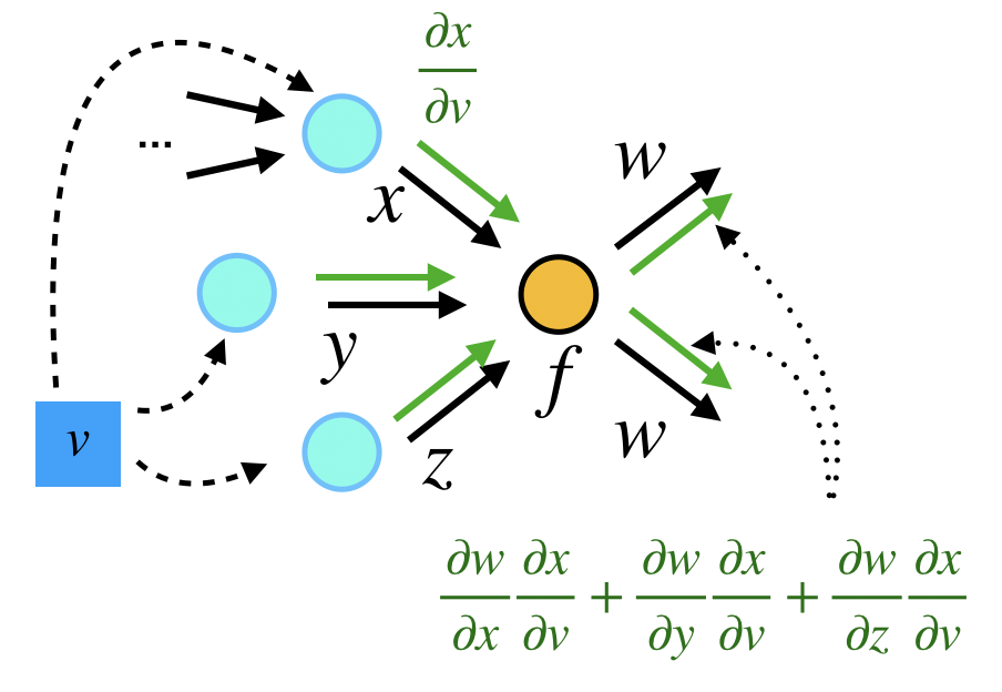
Forward Mode
In the forward mode, the gradients are computed in the same order as function evaluation, i.e.
$${\frac{\partial g'(x)}{\partial x}}$$
is computed first, and then
$$\frac{\partial f'\circ g(x)}{\partial g} {\frac{\partial g'(x)}{\partial x}}$$
as a whole. The idea is the same for a computational graph, except that we need to aggregate all the gradients from up-streams first, and then forward the gradients to down-stream nodes. Here we show how the gradient is computed:
$$f(x) = \begin{bmatrix} x^4\\ x^2 + \sin(x) \\ -\sin(x)\end{bmatrix}$$

Reverse Mode
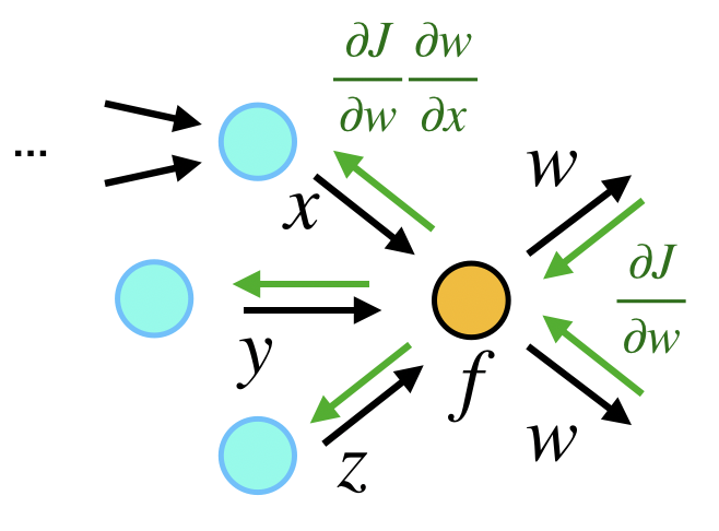
In contrast, the reverse-mode AD computes the gradient in the reverse order of forward computation, i.e.
$$\frac{\partial f'\circ g(x)}{\partial g}$$
is first evaluated and then
$$\frac{\partial f'\circ g(x)}{\partial g} {\frac{\partial g'(x)}{\partial x}}$$
as a whole. In the computational graph, each node first aggregate all the gradients from down-streams and then back-propagates the gradient to upstream nodes.
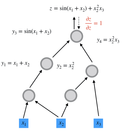
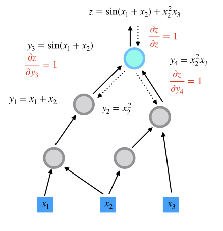
We show how the gradients of is evaluated:
$$z = \sin(x_1+x_2) + x_2^2 x_3$$
Reverse-mode AD in the Computational Graph
step 1
step 2
step 3
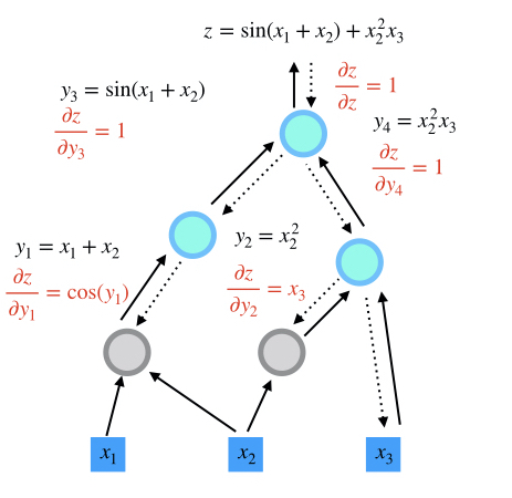
step 4
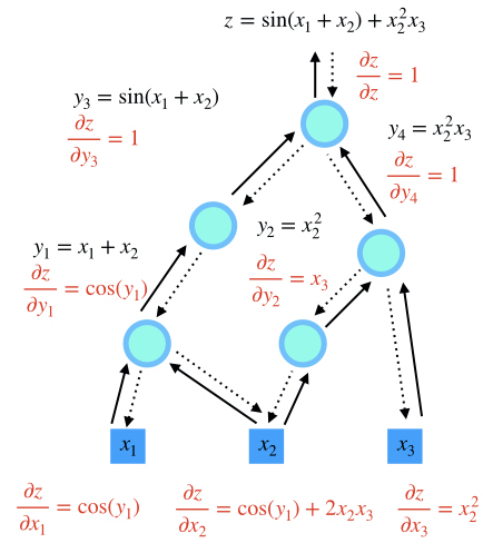
Comparison
Reverse-mode AD reuses gradients from down-streams. Therefore, this mode is useful for many-to-few mappings. In contrast, forward-mode AD reuses gradients from upstreams. This mechanism makes forward-mode AD suitable for few-to-many mappings. Therefore, for inverse modeling problems where the objective function is usually a scalar, reverse-mode AD is most relevant. For uncertainty quantification or sensitivity analysis, the forward-mode AD is most useful. We summarize the two modes in the following table:
For a function
$$f:\mathbf{R}^n \rightarrow \mathbf{R}^m$$

A Mathematical Description of Reverse-mode Automatic Differentiation
Because the reverse-mode automatic differentiation is very important for inverse modeling, we devote this section to a rigorious mathematical description of the reverse-mode automatic differentiation.
To explain how reverse-mode AD works, let's consider constructing a computational graph with independent variables
$$\{x_1, x_2, \ldots, x_n\}$$
and the forward propagation produces a single output
$$x_N, N>n$$
The gradients
$$\frac{\partial x_N(x_1, x_2, \ldots, x_n)}{\partial x_i}$$
he idea is that this algorithm can be decomposed into a sequence of functions
$$i=n+1, n+2, \ldots, N$$
that can be easily differentiated analytically, such as addition, multiplication, or basic functions like exponential, logarithm and trigonometric functions. Mathematically, we can formulate it as
$$\begin{aligned} x_{n+1} &= f_{n+1}(\mathbf{x}{\pi({n+1})})\\ x{n+2} &= f_{n+2}(\mathbf{x}{\pi({n+2})})\\ \ldots\\ x{N} &= f_{N}(\mathbf{x}_{\pi({N})})\\ \end{aligned}$$
where
$$\mathbf{x} = \{x_i\}_{i=1}^N$$
and π(i) are the parents of
$$\pi(i) \in \{1,2,\ldots,i-1\}$$
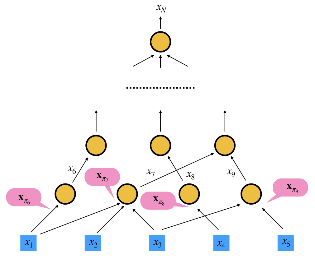

$$x_i(x_1, x_2, \ldots, x_{i-1}) = f_i(\mathbf{x}_{\pi(i)})$$

$$x_i(x_1, x_2, \ldots, x_j) = x_i(x_1, x_2, \ldots, x_j, f_{j+1}(\mathbf{x}_{\pi(j+1)})), \quad n < j+1 < i$$

$$x_N(x_1, x_2, \ldots, x_{N-1})$$

$$f_N(\mathbf{x}_{\pi(N)})$$

$$\frac{\partial x_N(x_1, x_2, \ldots, x_{i})}{\partial x_i} = \sum_{j\,:\,i\in \pi(j)} \frac{\partial x_N(x_1, x_2, \ldots, x_j)}{\partial x_j} \frac{\partial x_j(x_1, x_2, \ldots, x_{j-1})}{\partial x_i}$$

$$\frac{\partial x_j(x_1, x_2, \ldots, x_{j-1})}{\partial x_k}$$
is readily available since:
$$x_j(x_1, x_2, \ldots, x_{j-1}) = f_j(\mathbf{x}_{\pi(j)})$$
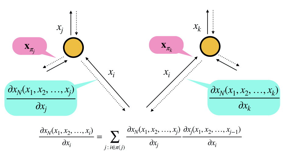

$$\frac{\partial x_N(x_1, x_2, \ldots, x_n)}{\partial x_i} = \sum_{j\,:\,i\in \pi(j)} \frac{\partial x_N(x_1, x_2, \ldots, x_j)}{\partial x_j} \frac{\partial x_j(x_1, x_2, \ldots, x_{j-1})}{\partial x_i}$$

$$\frac{\partial x_N(x_1, x_2, \ldots, x_j)}{\partial x_j}$$

step 1

step 2

step 3

step 4

TensorFlow
Google's TensorFlow provides a convenient way to specify the computational graph statically. TensorFlow has automatic differentiation features and its performance is optimized for large-scale computing. ADCME is built on TensorFlow by overloading numerical operators and augmenting TensorFlow with essential scientific computing functionalities. We contrast the TensorFlow implementation with the ADCME implementation of computing the objective function and its gradient in the following example.
$$y(x) = \|(AA^T+xI)^{-1}b-c\|^2, \; z = y'(x)$$

TensorFlow Implementation
import tensorflow as tf
import numpy as np
A = tf.constant(np.random.rand(10,10), dtype=tf.float64)
x = tf.constant(1.0, dtype=tf.float64)
b = tf.constant(np.random.rand(10), dtype=tf.float64)
c = tf.constant(np.random.rand(10), dtype=tf.float64)
B = tf.matmul(A, tf.transpose(A)) + x * tf.constant(np.identity(10))
y = tf.reduce_sum((tf.squeeze(tf.matrix_solve(B, tf.reshape(b, (-1,1))))-c)**2)
z = tf.gradients(y, x)[0]
sess = tf.Session()
sess.run([y, z])
Functions as Graphs
You must already be thinking of functions as “things” that take in stuff and spit out stuff. Rather than just “things”, let’s use a word that’s a bit more formal. How about “nodes” ?
A computational graph is a functional description of the required computation.
In the computational graph, an edge represents a value, such as a scalar, a vector, a matrix or a tensor. A node represents a function whose input arguments are the the incoming edges and output values are are the outcoming edges. Based on the number of input arguments, a function can be nullary, unary, binary, ..., and n-ary; based on the number of output arguments, a function can be single-valued or multiple-valued.
Computational graphs are directed and acyclic. The acyclicity implies the forward propagation computation is well-defined: we loop over edges in topological order and evaluates the outcoming edges for each node. To make the discussion more concrete, we illustrate the computational graph for
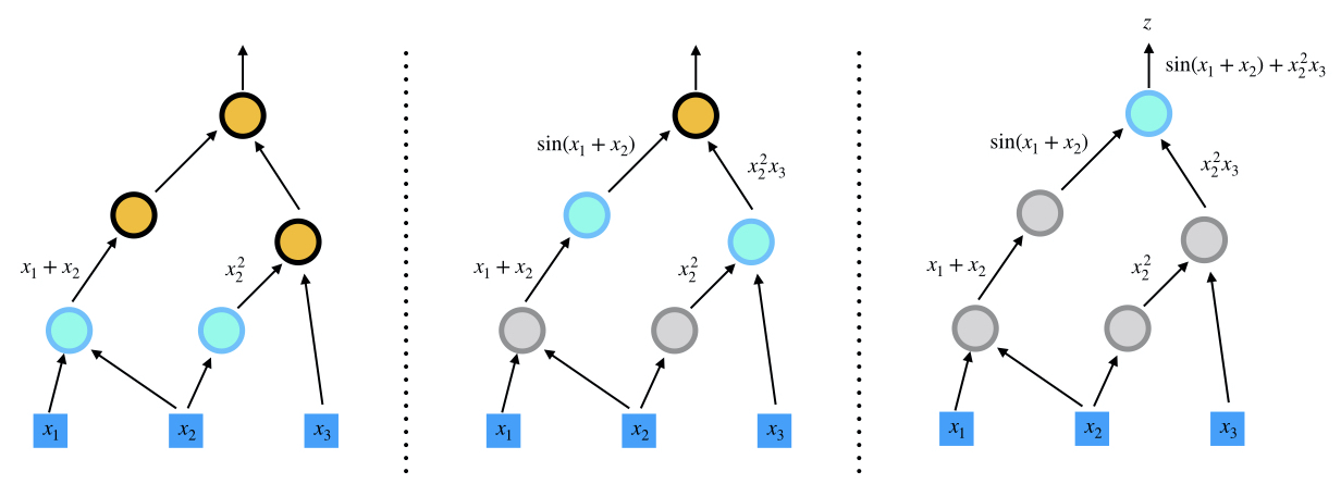
There are in general two programmatic ways to construct computational graphs: static and dynamic declaration. In the static declaration, the computational graph is first constructed symbolically, i.e., no actual numerical arithmetic are executed. Then a bunch of data is fed to the graph for the actual computation. An advantage of static declarations is that they allow for graph optimization such as removing unused branches. Additionally, the dependencies can be analyzed for parallel execution of independent components. Another approach is the dynamic declaration, where the computational graph is constructed on-the-fly as the forward computation is executed. The dynamic declaration interleaves construction and evaluation of the graph, making software development more intuitive.
Actually, each node will be slightly more than just the function. It’ll store all (or sufficiently many) of these things : the input values (t) , the output value (x), the gradient of the final function (f ) with respect to the output of the node and the gradient of the final function (f) with respect to the input values. Usually, at any instant we need to apply the chain rule, we’ll already know the gradient of final function (f) wrt output (x) and we can compute the gradient of output (x) wrt any of the inputs (t). Now, here’s where I make an important distinctions : the input to a node (seen as a variable) and the input node (also a variable) that the input is identical to, are actually separate entities.
This is because the input node could also be the input node of many other nodes, all of which will change on changing the value of the input node, but changing the value of the input doesn’t change the value of other nodes. Okay, enough details.
Simple, but fundamental functions, like addition, multiplication, etc. are what we can easily compute gradients for. So, once we implement these as nodes, we can implement complicated functions, like polynomials, sigmoid, etc. as graphs made of these nodes.
Simple, but fundamental functions, like addition, multiplication, etc. are what we can easily compute gradients for. So, once we implement these as nodes, we can implement complicated functions, like polynomials, sigmoid, etc. as graphs made of these nodes.
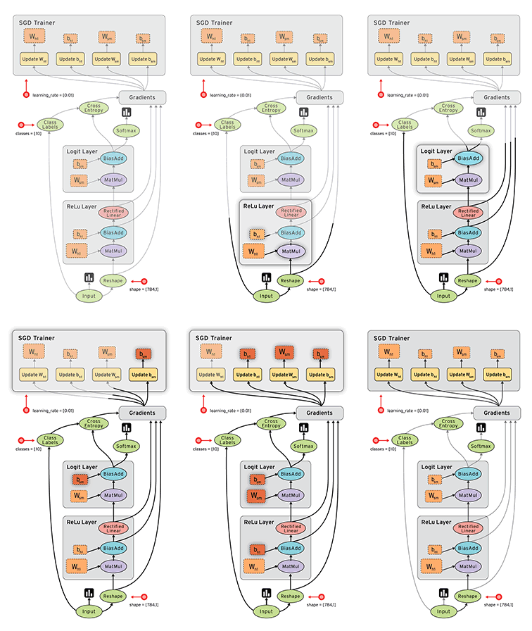
Okay, now equipped with this knowledge, let’s implement this in python :
from matplotlib.pyplot import *
from numpy import *
from numpy.linalg import eig
from graphviz import Digraph
from IPython.display import Image
from sklearn.datasets import load_breast_cancer

g = Digraph("Network")
NodeCollection = []
Variables = []
counter = 0
dt = 0.01
def Reset():
    global g,NodeCollection,Variables,counter,dt
    g = Digraph("Network")
    NodeCollection = []
    Variables = []
    counter = 0
    dt = 0.01
class Node:
    name = None
    COLOR = "black"
    def __init__(self,name=None,draw=True):
        global counter,NodeCollection
        self.value = None
        self.outputNodes = []
        self.inputNodes = []
        self.id = counter
        self.draw = draw
        if self.name==None and name == None:
            self.name = "node "+str(self.id)
        elif name!=None:
            self.name = name
        if draw:
            g.node(str(self.id),self.name,color=self.COLOR)
        NodeCollection.append(self)
        counter += 1
    def __repr__(self):
        return f"name : {self.name}\n value : \n{self.value}\n grad : \n{self.grad}\n"
    def __add__(self,other):
        return Add([self,toNode(other)],"+")
    def __mul__(self,other):
        return Mul([self,toNode(other)],"*")
    def __pow__(self,other):
        return Pow([self,toNode(other)],"**")
    def __div__(self,other):
        return self*(other**(-1))
    def __neg__(self):
        return Neg([self],"-")
    def __sub__(self,other):
        return self + (-toNode(other))
    def recieve(self):
        self.grad = 0
        for n in self.outputNodes:
            DFDX = n.dfdx_value[self.id]
            GRAD = n.grad
            #print("recievong from",n.id,"aka",n.name)
            #print("DFDX",DFDX.shape)
            #print("GRAD",GRAD.shape)
            if len(DFDX.shape)==1 and GRAD.shape==(1,DFDX.shape[0]) and len(self.value.shape)==2:
                self.grad += GRAD.T @ DFDX[newaxis,:]
            elif DFDX.shape==(1,) or GRAD.shape ==(1,):
                self.grad += GRAD*DFDX
            else:
                #self.grad += dot(GRAD,DFDX)
                self.grad += GRAD @ DFDX
class Function(Node):
    COLOR = "green"
    f = None
    dfdx = None
    dfdx_value = None
    def __init__(self,inputNodes,name=None,draw=True):
        super().__init__(name,draw)
        for n in inputNodes:
            if self.draw and n.draw:
                g.edge(str(n.id),str(self.id))
            n.outputNodes.append(self)
        self.inputNodes = inputNodes
        self.forward()
    def __repr__(self):
        return f"name : {self.name}\n value : \n{self.value}\n grad : \n{self.grad}\n dfdx : \n{self.dfdx_value}\n"
    def forward(self):
        self.inputs = dict([(node.id,node.value) for node in self.inputNodes])
        self.value = self.f(self.inputs)
        self.dfdx_value = self.dfdx(self.inputs)
        n = int(prod(self.value.shape))
        #if n > 1:
        #    self.grad = identity(n)
        #else :
        #    self.grad = array(1)
        self.grad = identity(n)
    def backward(self):
        for n in self.inputNodes:
            n.recieve()
            n.backward()
class Variable(Node):
    COLOR = "red"
    def __init__(self,value,name=None,draw=True):
        super().__init__(name,draw)
        self.value = value
        n = prod(self.value.shape)
        self.grad = identity(n)
        Variables.append(self)
    def backward(self):
        pass
    def forward(self):
        global dt
        self.grad.resize(self.value.shape)
        self.value = self.value - self.grad*dt
class Constant(Variable):
    COLOR="black"
    def recieve(self):
        pass
    def forward(self):
        pass
def toNode(other,draw=True):
    name = None
    if isinstance(other,Node):
        return other
    if type(other) != ndarray:
        if type(other) != iterable:
            name = str(other)
            other = array([other])
        else:
            other = array(other)
    return Constant(other,name,draw)
Now, let’s add some fundamental functions:
class Add(Function):
    name = "+"
    def f(self,inputs):
        S = 0
        for id in inputs:
            S = S + inputs[id]
        return S
    def dfdx(self,inputs):
        G = dict()
        for id in inputs:
            n = prod(inputs[id].shape)
            if n>1:
                G[id] = identity(n)
            else:
                G[id] = ones(prod(self.value.shape))[:,newaxis]
        return G
class Mul(Function):
    name = "*"
    def f(self,inputs):
        S = 1
        for id in inputs:
            S = S*inputs[id]
        return S
    def dfdx(self,inputs):
        G = dict()
        for id in inputs:
            S = 1
            for Id in inputs:
                if Id == id:
                    continue
                S = S*inputs[Id]
            S = S.flatten()
            n = prod(inputs[id].shape)
            if n > 1:
                m, = S.shape
                if m > 1:
                    S = diag(S)
                else :
                    S = S * identity(n)
            else:
                S = S[:,newaxis]
            G[id] = S
        return G
class Exp(Function):
    name = "exp"
    def f(self,inputs):
        return exp(next(iter(inputs.values())))
    def dfdx(self,inputs):
        id = next(iter(inputs.keys()))
        x = next(iter(inputs.values()))
        n = prod(x.shape)
        x = exp(x)
        x = x.flatten()
        if n>1:
            return {id:diagflat(x)}
        return {id:x[:,newaxis]}
class Pow(Function):
    name = "**"
    def f(self,inputs):
        x,n = inputs.values()
        return x**n
    def dfdx(self,inputs):
        ids = list(inputs.keys())
        x,n = inputs.values()
        m = prod(x.shape)
        if m > 1:
            return {ids[0]:diagflat(n*x**(n-1))}#,ids[1]:(log(x)*x**n).flatten()[:,newaxis]}
        return {ids[0]:(n*x**(n-1)).flatten()[:,newaxis]}#,ids[1]:(log(x)*x**n).flatten()[:,newaxis]}
class Neg(Function):
    name = "-"
    def f(self,inputs):
        return -next(iter(inputs.values()))
    def dfdx(self,inputs):
        id = next(iter(inputs.keys()))
        x = next(iter(inputs.values()))
        n = int(prod(x.shape))
        #if n>1:
        #    return {id:-identity(n)}
        #return {id:-array([1])}
        return {id:-identity(n)}
class Dot(Function):
    name = "."
    def f(self,inputs):
        x,y = inputs.values()
        d = dot(x,y)
        if len(d.shape)>0:
            return d
        return array([d])
    def dfdx(self,inputs):
        id1,id2 = inputs.keys()
        x,y = inputs.values()
        if len(x.shape) == 1:
            x = x[newaxis,:]
            y = y[newaxis,:]
        return {id1:y,id2:x}
class Sum(Function):
    name = "sum"
    def f(self,inputs):
        x, = inputs.values()
        return array([sum(x)])
    def dfdx(self,inputs):
        x, = inputs.values()
        id, = inputs.keys()
        n = prod(x.shape)
        return {id:ones((1,n))}
class Sin(Function):
    name = "sin"
    def f(self,inputs):
        x, = inputs.values()
        return sin(x)
    def dfdx(self,inputs):
        x, = inputs.values()
        id, = inputs.keys()
        n = prod(x.shape)
        return {id:diagflat(cos(x))}
class Cos(Function):
    name = "cos"
    def f(self,inputs):
        x, = inputs.values()
        return cos(x)
    def dfdx(self,inputs):
        x, = inputs.values()
        id, = inputs.keys()
        n = prod(x.shape)
        return {id:diagflat(sin(x))}
class MatFunc(Function):
    def forward(self):
        self.inputs = dict([(node.id,node.value) for node in self.inputNodes])
        self.value = self.f(self.inputs)
        n = int(prod(self.value.shape))
        self.grad = identity(n)
    def __init__(self, inputNodes, name=None, draw=True):
        super().__init__(inputNodes, name, draw)
        for n in self.inputNodes:
            if isinstance(n,MatFunc):
                n.recieve = n.send
            else:
                n.recieve = lambda:None
    def recieve(self):
        super().recieve()
        self.send()
class MatMul(MatFunc):
    name = "@"
    def f(self,inputs):
        W,X = inputs.values()
        return W @ X
    def send(self):
        w,x = self.inputNodes
        W = w.value
        X = x.value
        G = self.grad
        w.grad = G @ X.T
        x.grad = W.T @ G
class SigmM(MatFunc):
    name = "Sigma"
    def f(self,inputs):
        X, = inputs.values()
        return sigmoid(X)
    def send(self):
        x, = self.inputNodes
        X = x.value
        G = self.grad
        sig = sigmoid(X)
        x.grad = G*(sig**2/exp(X))
class SqNorM(MatFunc):
    name = "Norm"
    def f(self,inputs):
        X, = inputs.values()
        return array([linalg.norm(X,'fro')])**2
    def send(self):
        x = self.inputNodes[0]
        x.grad = 2*x.value*self.grad
class DotM(MatFunc):
    name = "."
    def f(self,inputs):
        X,Y = inputs.values()
        return sum(X*Y)
    def send(self):
        x,y = self.inputNodes
        X,Y = x.value,y.value
        G = self.grad # assumed to be a scalar
        x.grad = Y*G
        y.grad = X*G
class AddM(MatFunc):
    name = "+"
    def f(self,inputs):
        S = 0
        for X in inputs.values():
            S = S + X
        return S
    def send(self):
        for n in self.inputNodes:
            if len(n.value.shape) == 1 or n.value.shape[0] == 1:
                n.grad = sum(self.grad,axis=0)
            else :
                n.grad = self.grad
class NegM(MatFunc):
    name = "-"
    def f(self,inputs):
        X, = inputs.values()
        return -X
    def send(self):
        x = self.inputNodes[0]
        x.grad = -self.grad
Back Propagation
Remember what we are doing all of this for. We want to do gradient descent on the nodes that are not dependent on any other nodes. We know we can calculate the gradient of f wrt the value of a node, given all the output nodes have the latest value of the gradient wrt their value. This means, we must compute these values in the reverse topological order (order of creation, in this case) . And, of course, for computing the outputs of the nodes, we need to move in forward order. The first process is called “back propagation” . Similarly, I name the 2nd process as “forward propagation” .
def BacProp(show=False):
    global NodeCollection
    for i in range(len(NodeCollection)-2,-1,-1):
        n=NodeCollection[i]
        n.recieve()
        if show:
            print(n)
def forProp(show=False):
    global NodeCollection
    for i in range(len(NodeCollection)):
        n=NodeCollection[i]
        n.forward()
        if show:
            print(n)
def Descend(iterations=100):
    global dt,NodeCollection,Variables
    L = NodeCollection[-1]
    print("before",L.value)
    for i in range(iterations):
        BacProp()
        forProp()
    print("after",L.value)
In fact, with all of this, we are in a position to build a small neural network right away. First, let’s make a perceptron.
Perceptron
It’s a function that outputs the sigmoid of a linear combination of different features (nodes in preceding layer) . The weights are variables (hyperparameters really). There’s a lot of information on this topic as well, so I’ll just shut up and show you the code.
def Sigm(inputNode,name="S",draw=True):
    out = Neg([inputNode],None,False)
    out = Exp([out],None,False)
    out = Add([out,Constant(array([1]),None,False)],None,False)
    out = Pow([out,Constant(array([-1]),None,False)],name,True)
    if draw and inputNode.draw:
        g.edge(str(inputNode.id),str(out.id))
    return out
def perceptron(layer,draw=True):
    nl = []
    for n in layer :
        nl.append(Mul([n,Variable(random.random(1),None,False)],None,False))
    S = Add(nl,"+",False)
    S = Sigm(S,"P",draw)
    for n in layer:
        if draw and n.draw:
            g.edge(str(n.id),str(S.id))
    S.nl = nl
    return S
Loss function
Let’s also make a function that gives the Euclidian norm between two vectors. This is what’s called a loss function (there are many varieties) which tells us how bad was our prediction.
def SqEr(inputNodes,name="L",draw=True):
    x,y = inputNodes
    out = Neg([y],None,False)
    out = Add([x,out],None,False)
    two = Constant(array([2]),None,False)
    out = Pow([out,two],None,False)
    out = Sum([out],name,draw)
    for n in inputNodes:
        if draw and n.draw:
            g.edge(str(n.id),str(out.id))
    return out
Neural Net
And finally, let’s make the whole neural net.
class PerceptronNet:
    def __init__(self,LS=[3,3,3]):
        Reset()
        n = LS.pop(0)
        layer0 = [Constant(ones(1)) for _ in range(n)]
        layers = [layer0]
        for n in LS:
            last_layer = layers[-1]
            layers.append([perceptron(last_layer) for _ in range(n)])
        P = perceptron(layers[-1])
        y = Constant(ones(1),"y")
        L = SqEr([P,y])
        self.y = y
        self.layer0 = layer0
        self.P = P
        self.L = L
        self.layers = layers
    def assign(self,X,y):
        if X.shape[1]!= len(self.layer0):
            print("Can't deal with this many variables.")
            return
        self.y.value = y
        for c in range(X.shape[1]):
            self.layer0[c].value = X[:,c]
        forProp()
    def predict(self):
        forProp()
        loss = self.L.value
        y_pred = self.P.value
        return y_pred,loss
Usage
We can use this on the breast cancer dataset like this :
X,y = load_breast_cancer(return_X_y=True)

# PCA
mu = mean(X,0)
sd = var(X,0)**0.5
X = (X-mu)/sd
## Assume X = Y @ R.T and Y.T @ Y = D
C = X.T @ X
D,RT = eig(C)
idx = argsort(D)[-7:]
D = D[idx]
RT = RT[:,idx]
X = X @ RT
X = real(X)

#Neural Net
net = PerceptronNet([7,5])
net.assign(X,y)
dt = 0.001
print(mean(around(net.P.value)==net.y.value)*100)
Descend(100)
print(mean(around(net.P.value)==net.y.value)*100)
Show(g,200)
This gives this graph :
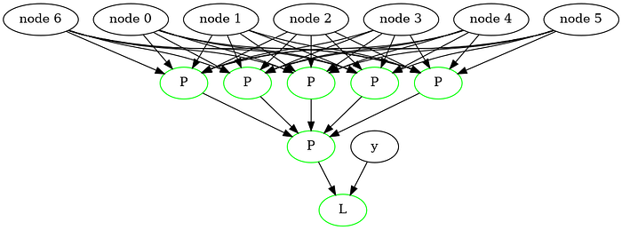
And an accuracy of 90-95% on the training data itself. We can increase this drastically by descending for longer. But to do that, we need a more efficient model. This can be done by using matrices for layers, rather than individual perceptrons.
Layers as Matrices
def Layer(X,pin,pout,name=None,bias=False):
    W = random.random((pin,pout))
    W = Variable(W,"W")
    Y = MatMul([X,W])
    if bias:
        b = random.random(pout)
        b = Variable(b,"b")
        Y = AddM([Y,b])
    Y = SigmM([Y],name)
    return Y
def SqErM(inputNodes):
    yp,y = inputNodes
    myp = NegM([yp])
    er = AddM([myp,y])
    s = SqNorM([er],"L")+0
    return s
class LayerNet:
    def __init__(self,X,y,middle=[3,3,3],bias=False,normalise=False):
        if isinstance(bias,bool):
            bias = [bias for _ in range(len(middle))]
        Reset()
        m = X.shape[1]
        n = y.shape[1]
        mu = mean(X,axis=0)
        sdi = diag(var(X,axis=0)**(-0.5))
        X = Constant(X,"X")
        y = Constant(y,"y")
        self.y = y
        self.X = X
        if normalise:
            nmu = Constant(-mu,'b')
            sdi = Constant(sdi,"W")
            X = AddM([X,nmu],"shifted X")
            X = MatMul([X,sdi],"normalised X")
        out = Layer(X,m,middle[0],"layer1",True)
        for i in range(len(middle)-1):
            out = Layer(out,middle[i],middle[i+1],f"layer {i+1}",bias[i])
        y_pred = Layer(out,middle[-1],n,'y_pred',bias[-1])
        L = SqErM([y_pred,y])
        self.y_pred = y_pred
        self.L = L
    def predict(self,X,y,testName = ""):
        self.X.value = X
        self.y.value = y
        forProp()
        y_pred = self.y_pred.value
        print("accuracy on test ",testName," : ",round(mean(around(y_pred)==y)*100,2),"%")
        return y_pred
    def train(self,iterations=100,dtvalue=0.01):
        global dt
        dtold = dt
        dt = dtvalue
        y_pred = self.y_pred.value
        y = self.y.value
        print("accuracy before training : ",round(mean(around(y_pred)==y)*100,2),"%")
        Descend(iterations)
        dt = dtold
        y_pred = self.y_pred.value
        y = self.y.value
        print("accuracy on training : ",round(mean(around(y_pred)==y)*100,2),"%")
Using this for the breast cancer dataset, without even doing PCA, we get 96–98% accuracy on a testing data
X,y = load_breast_cancer(return_X_y=True)
m = X.shape[1]
X = X[:]
y = y[:,newaxis]
X,Xtest = X[:300,:],X[300:,:]
y,ytest = y[:300,:],y[300:,:]

net = LayerNet(X,y,[5],normalise=True)
net.train(100,0.01)
net.predict(Xtest,ytest)
Show(g)
This looks like this :
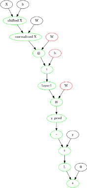
Now, you might think that neural networks aren’t so good after all, since we got only 96–98% accuracy. Well, the thing is, I chose the wrong activation function and loss function. We usually use the sigmoid and squared error for regression tasks. In this case, we want to perform a classification task, for which we should use the soft-max activation function and cross entropy loss function. Using that and 2 hidden layers with 10 and 3 perceptrons, we get this output :
accuracy before training : 48.67 %
before [2.77841405]
after [0.00597004]
accuracy on training : 100.0 %
accuracy on test : 96.28 %
Choi RY, Coyner AS, Kalpathy-Cramer J, Chiang MF, Campbell JP. Introduction to Machine Learning, Neural Networks, and Deep Learning. Transl Vis Sci Technol. 2020 Feb 27;9(2):14. doi: 10.1167/tvst.9.2.14. PMID: 32704420; PMCID: PMC7347027.
Kriegeskorte N, Golan T. Neural network models and deep learning. Curr Biol. 2019 Apr 1;29(7):R231-R236. doi: 10.1016/j.cub.2019.02.034. PMID: 30939301.
Shao F, Shen Z. How can artificial neural networks approximate the brain? Front Psychol. 2023 Jan 9;13:970214. doi: 10.3389/fpsyg.2022.970214. PMID: 36698593; PMCID: PMC9868316.
Aijaz J. Why medical professionals must learn mathematics and computing? Pak J Med Sci. 2024 Jan;40(2ICON Suppl):S106. doi: 10.12669/pjms.40.2(ICON).8952. PMID: 38328646; PMCID: PMC10844920.
Lee, N., & Cichocki, A. (2014). Fundamental Tensor Operations for Large-Scale Data Analysis in Tensor Train Formats. ArXiv, abs/1405.7786.
E. Karahan, P. A. Rojas-López, M. L. Bringas-Vega, P. A. Valdés-Hernández and P. A. Valdes-Sosa, "Tensor Analysis and Fusion of Multimodal Brain Images," in Proceedings of the IEEE, vol. 103, no. 9, pp. 1531-1559, Sept. 2015, doi: 10.1109/JPROC.2015.2455028.
Caiafa, C.F.; Solé-Casals, J.; Marti-Puig, P.; Zhe, S.; Tanaka, T. Decomposition Methods for Machine Learning with Small, Incomplete or Noisy Datasets. *Appl. Sci.*2020, 10, 8481. doi.org/10.3390/app10238481.
Rosenblatt, F. The perceptron: A probabilistic model for information storage and organization in the brain. Psychol. Rev. 1958, 65, 386.
Chen, Chi & Zuo, Yunxing & Ye, Weike & Li, Xiang-Guo & Deng, Zhi & Ong, Shyue. (2020). A Critical Review of Machine Learning of Energy Materials. Advanced Energy Materials. 1903242. 10.1002/aenm.201903242.
Zheng, P., Zubatyuk, R., Wu, W. et al. Artificial intelligence-enhanced quantum chemical method with broad applicability. Nat Commun**12**, 7022 (2021). doi.org/10.1038/s41467-021-27340-2
Lecun, L. Bottou, Y. Bengio and P. Haffner, "Gradient-based learning applied to document recognition," in Proceedings of the IEEE, vol. 86, no. 11, pp. 2278-2324, Nov. 1998, doi: 10.1109/5.726791.
Li, X.; Ma, X.; Xiao, F.; Wang, F.; Zhang, S. Application of Gated Recurrent Unit (GRU) Neural Network for Smart Batch Production Prediction. Energies**2020*, 13*, 6121. doi.org/10.3390/en13226121
Chung, J., Gulcehre, C., Cho, K., & Bengio, Y. (2014). Empirical evaluation of gated recurrent neural networks on sequence modeling. In NIPS 2014 Workshop on Deep Learning, December 2014
G. E. Hinton and T. J. Sejnowski. 1986. Learning and relearning in Boltzmann machines. Parallel distributed processing: explorations in the microstructure of cognition, vol. 1: foundations. MIT Press, Cambridge, MA, USA, 282–317.
Bengio, Y. & Lamblin, Pascal & Popovici, Dan & Larochelle, Hugo. (2007). Greedy layer-wise training of deep networks. Adv. Neural Inf. Process. Syst.. 19. 153-160.
Luo, Tony & Nagarajany, Sai. (2018). Distributed Anomaly Detection Using Autoencoder Neural Networks in WSN for IoT. 1-6. 10.1109/ICC.2018.8422402.
Bourlard H, Kamp Y. Auto-association by multilayer perceptrons and singular value decomposition. Biol Cybern. 1988;59(4-5):291-4. doi: 10.1007/BF00332918. PMID: 3196773.
Goodfellow, Ian & Pouget-Abadie, Jean & Mirza, Mehdi & Xu, Bing & Warde-Farley, David & Ozair, Sherjil & Courville, Aaron & Bengio, Y.. (2014). Generative Adversarial Networks. Advances in Neural Information Processing Systems. 3. 10.1145/3422622.
Hopfield, John. (1982). Neural Networks and Physical Systems with Emergent Collective Computational Abilities. Proceedings of the National Academy of Sciences of the United States of America. 79. 2554-8. 10.1073/pnas.79.8.2554.
