Neural Networks Lectures Introduction


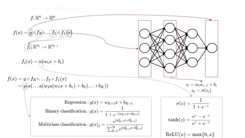
Based on a given dataset, a neuronal network creates a function f which maps the relationship between features Xi and labels Y. The advantage of deep learning is that it automates feature engineering. At their core, neural networks consist of interconnected neurons that process and transform data. Information is passed into the network, and as it propagates through layers of neurons, complex relationships between input and output are learned. Each connection between neurons carries a weight that determines the strength of their influence on the data’s transformation.
For any arbitrary function f there exist a neuronal network. The goal is to find the best parameters 𝜃 (weights) which result in the best decision boundary.
Let’s consider the illustrations below:
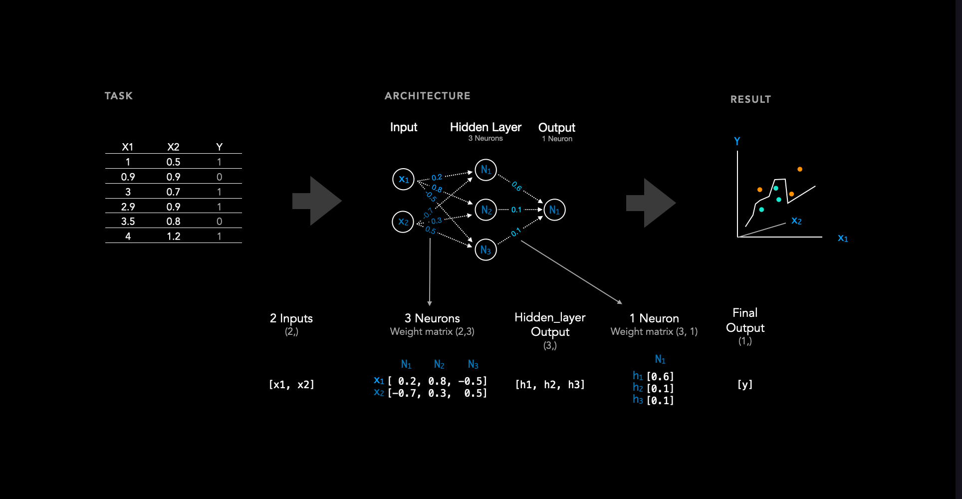
As we can see, there is a dataset on the left. Typically, the dataset consists of some features denoted as x. In this case, we have two features, x1 and x2, for each sample. Additionally, there is a label, also referred to as the target or class, associated with each sample.
To learn the relationship between features X1 and X2 and their corresponding label, we utilize a neural network consisting of 2 input nodes (owing to the two features), one hidden layer with 3 neurons (the number of hidden layers and neurons can be adjusted as hyperparameters), and one output neuron. A weight matrix is associated with each layer. In this instance, there exists a hidden layer and an output layer, resulting in two weight matrices. These weights are initialized randomly, and throughout the training process, they are iteratively updated until the loss converges. A weight matrix always has the dimension n x m
nneurons in the previous layer (input layer or a previous hidden layer).mneurons in the current hidden layer.
After training a neural network, a decision boundary is obtained. If we then introduce a sample that was not included in the training data, the neural network classifies the new, unseen datapoint based on this decision boundary.
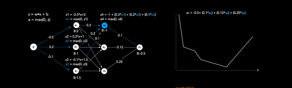
The prediction of input in a neural network (Forward pass)
Figure 2 illustrates how input data is passed forward in a neural network with only one output node (a7) that can be used for regression tasks (In this case we use arbitrary weights and biases for illustration purposes, thus the prediction would be nonsense). The illustration shows how a neural network results in a specific function. Each node in a hidden layer has the following function: z = a(weights*input+bias), where a refers to an activation function, such as ReLu. The last node a7 is a combination of all previous functions, resulting in one single non-linear function. To understand the combination of functions, we can take node a4 as an example. We can see that node a4 depends on the functions of nodes a1 to a3, which in turn depend on the input x. In particular, the value of node a4 is calculated by a(weights*input+bias). In this case the bias is -1, the weights are 0.3, 0.2 and 0.1. And the input is the output of the previous three nodes a1,a2 and a3.
In this illustration we use ReLU as activation function, which simply is max(0, z).
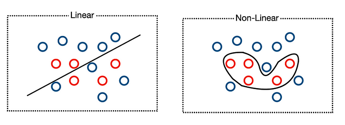
Activation Functions
Activation functions are important because they introduce non-linearity. Thus complex non-linear decision boundaries can be accomplished.

ReLu is a common choice for hidden layer activation. It is computationally efficient, because it uses only a simple thresholding operation. It is less susceptible to vanishing gradient problem because the gradients are 1 if x>0. However, every negative value results in a gradient of zero, which means the weights will never be updated, resulting in a dead neuron.
The Sigmoid activation function compresses values between 0 and 1, which can be interpreted as a probability that the input belongs to a specific class. It is frequently employed as an activation function for the output in binary classification problems. However, the Sigmoid function yields very small gradients that can lead to neural network stagnation. Additionally, it causes gradients to vanish beyond 1 and 0, respectively.
Different Network Architectures and Loss Functions
The network architecture differs depending on the task. In general, one distinguishes between regression, binary classification and categorical classification tasks. The loss function depends on the task.
Binary Classification
If we want to classify an input only into two options, class 1 or class 0, we use an architecture similar to the one illustrated below.

It is important to note that we only have one output node in binary classification tasks. This output node uses the sigmoid activation function, which squeezes values between 0 and 1.
We use sigmoid, because the output value close to 1 can be interpreted as a high probability of the input belonging to one class, while an output value close to 0 indicates a high probability of belonging to the other class.
Binary Cross-Entropy Loss
$$-{(y\log(p) + (1 - y)\log(1 - p))} -\sum_{c=1}^My_{o,c}\log(p_{o,c})$$
Because our weights are initialised randomly at the beginning, the first prediction will be completely nonsense. Binary cross-entropy loss is a loss function that helps us to understand how bad the prediction was by measuring the dissimilarity between predicted probabilities and the actual target values.
Binary Cross-Entropy Loss:
L = - (y_true * log(y_pred) + (1 - y_true) * log(1 - y_pred) )
In Figure 4 we see that the prediction for the first sample was 0.7 and the target was 1. If we pass this into the binary cross-entropy loss function we get a loss of 0.15:
L = - (1 * log(0.7) + (1 - 1) * log(1 - 0.7) )
  = - log(0.7)
  = 0.15
Similarly, the second sample yields the prediction 0.4 and the target was 0, thus the loss is 0.2:
L = - (0 * log(0.4) + (1 - 0) * log(1 - 0.4) )
  = - log(1-0.4)
  = 0.2
Multi-Class classification
If we want to classify an input that has more than two target classes, we use an architecture that has one output neuron for each class.
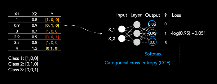
First, of all we have to encode all labels as one-hot-encode, thus, if we have three classes we have an array of size three, as label for each class.
The last layer uses softmax instead of sigmoid. Softmax function is typically used in multi class classification problems. It is applied to the outputs of all nodes in the output layer of a neural network. The output of the function is a vector of values between 0 and 1 that sum to 1.
For the loss we only select the predicted probabilities for the true classes for each sample and take the negative log of that predicted probability. The loss is averaged over all samples.
Regression
In regression, we have only one output node and no activation function. As Loss function we use mean-squared error.
$$\sum_{i=1}^{D}(x_i-y_i)^2$$
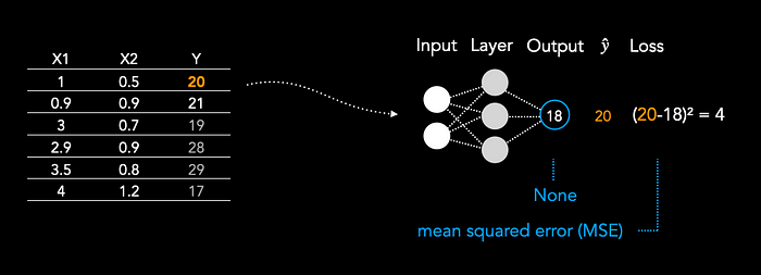
Mean-squared error:
L = (y_true - y_pred)²
MSE penalizes larger prediction errors more significantly due to the squaring operation. This means that outliers or instances with larger errors contribute more to the overall loss. Minimizing MSE during training encourages the model to adjust its parameters to make predictions that closely match the actual target values, resulting in a regression model that provides accurate estimations.
Bibliography
Choi RY, Coyner AS, Kalpathy-Cramer J, Chiang MF, Campbell JP. Introduction to Machine Learning, Neural Networks, and Deep Learning. Transl Vis Sci Technol. 2020 Feb 27;9(2):14. doi: 10.1167/tvst.9.2.14. PMID: 32704420; PMCID: PMC7347027.
Kriegeskorte N, Golan T. Neural network models and deep learning. Curr Biol. 2019 Apr 1;29(7):R231-R236. doi: 10.1016/j.cub.2019.02.034. PMID: 30939301.
Shao F, Shen Z. How can artificial neural networks approximate the brain? Front Psychol. 2023 Jan 9;13:970214. doi: 10.3389/fpsyg.2022.970214. PMID: 36698593; PMCID: PMC9868316.
Aijaz J. Why medical professionals must learn mathematics and computing? Pak J Med Sci. 2024 Jan;40(2ICON Suppl):S106. doi: 10.12669/pjms.40.2(ICON).8952. PMID: 38328646; PMCID: PMC10844920.