Machine learning algorithms appear to operate in a realm of complexity, but beneath the surface lies a foundation built upon the elegant principles of linear algebra. This lecture delves into these fundamental concepts and explores their seamless integration with machine learning, showcasing the practical implementation through Python code.

Building Blocks: Unveiling the Language of Linear Algebra

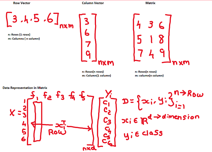
Vectors: Ordered sequences of numbers representing data points. Imagine a point in space with coordinates (x, y, z). Each coordinate is a component of the vector. We can represent a vector mathematically as:

$$v = [v₁, v₂, ..., vₙ]$$

Matrices: Rectangular arrangements of numbers used for storing and manipulating data. They can be visualized as grids, where each entry represents an intersection point. Mathematically, a matrix is denoted as:

$$A = [[a₁₁, a₁₂, ..., a₁ₙ], [a₂₁, a₂₂, ..., a₂ₙ], ..., [aₘ₁, aₘ₂, ..., aₘₙ]]$$

Example (Python Implementation):

# Define a vector
vector = [1, 2, 3]

# Define a matrix
matrix = [[1, 2], [3, 4]]

# Access elements: vector[0] = 1, matrix[0][1] = 2

Operations: The Powerful Tools of Linear Algebra

Vector Addition/Subtraction: Add/subtract corresponding elements of equal-sized vectors. Mathematically, for vectors u and v:

$$u + v = [u₁ + v₁, u₂ + v₂, ..., uₙ + vₙ]$$

$$u - v = [u₁ - v₁, u₂ - v₂, ..., uₙ - vₙ]$$

Matrix Addition/Subtraction: Add/subtract corresponding elements of matrices with the same dimensions. Mathematically, for matrices A and B:

$$A + B = [[a₁₁ + b₁₁, a₁₂ + b₁₂, ..., a₁ₙ + b₁ₙ], [a₂₁ + b₂₁, a₂₂ + b₂₂, ..., a₂ₙ + b₂ₙ], ..., [aₘ₁ + bₘ₁, aₘ₂ + bₘ₂, ..., aₘₙ + bₘₙ]]$$

Scalar Multiplication: Multiply each element of a vector or matrix by a constant scalar value c:

Matrix Multiplication: Defined operation combining two matrices to produce a new matrix. The resulting dimensions depend on the dimensions of the input matrices. Mathematically, for matrices A (m x n) and B (p x q):

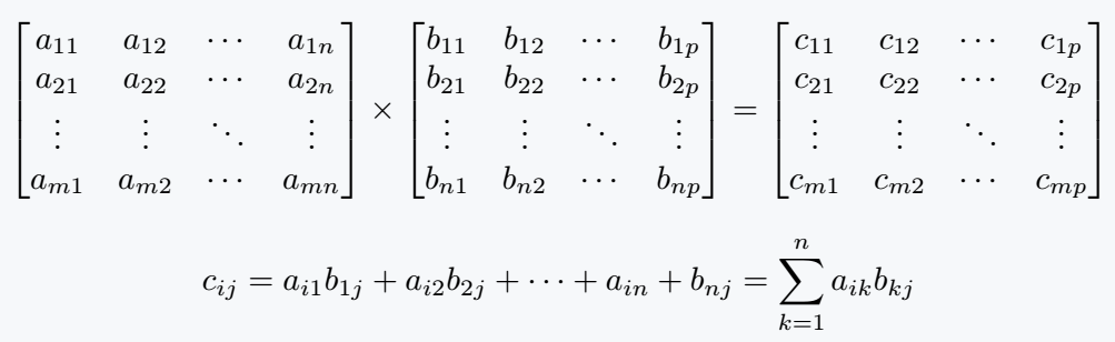
Example (Python Implementation using NumPy):

# Import library
import numpy as np

# Define matrices
A = np.array([[1, 2], [3, 4]])
B = np.array([[5, 6], [7, 8]])

# Addition, subtraction, scalar multiplication
C = A + B
D = A - B
E = 2 * A

# Matrix multiplication
F = np.dot(A, B)  # Using NumPy's dot product for matrix multiplication

Representation of Data

One of the fundamental applications of matrices and vectors in machine learning is the representation of data. In most machine learning tasks, data is typically organized in a tabular format, where each row represents an observation and each column represents a feature or attribute. This tabular structure can be represented as a matrix, where each element corresponds to a specific value in the dataset.

The fuel of ML models, that is data, needs to be converted into arrays before you can feed it into your models. The computations performed on these arrays include operations like matrix multiplication (dot product). This further returns the output that is also represented as a transformed matrix/tensor of numbers.

For example, consider a dataset of housing prices with features such as the number of bedrooms, square footage, and location. This dataset can be represented as an m x n matrix, where m is the number of observations (rows) and n is the number of features (columns). Each element in the matrix represents the value of a specific feature for a particular observation.

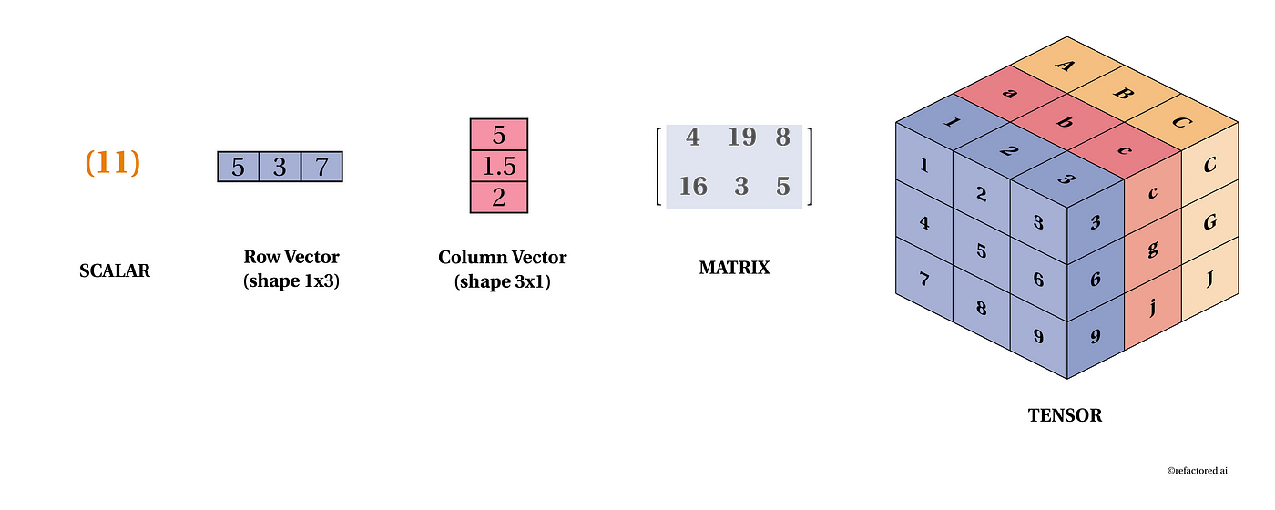
Linear algebra basically deals with vectors and matrices (different shapes of arrays) and operations on these arrays. In NumPy, vectors are basically a 1-dimensional array of numbers but geometrically, they have both magnitude and direction.Our data can be represented using a vector. In the figure below, one row in this data is represented by a feature vector which has 3 elements or components representing 3 different dimensions. N-entries in a vector makes it n-dimensional vector space and in this case, we can see 3-dimensions.

In the context of data science, particularly in machine learning, the significance of linear algebra becomes evident when dealing with datasets that have numerous features, making visualization and manual judgment challenging. While we can easily visualize and draw lines in 2 or 3-dimensional Cartesian space, real-world datasets often involve a high-dimensional space (N-dimensions) that is impractical to visualize. This is where the power of linear algebra comes into play. It allows us to apply mathematical principles to machine learning models, enabling the creation of decision boundaries or planes in N-dimensional space for accurate data classification and analysis.

Data representation includes transforming data into vectors and matrices, which are structured mathematical objects that can be manipulated to perform operations like addition, multiplication, and transformation.

Linear Algebra in Data Preprocessing

Data preprocessing in the context of linear algebra involves various techniques and operations applied to raw data to make it suitable for analysis, modeling, or other mathematical operations using linear algebra: Data Scaling, Normalization, Standardization, Robust Scaling.

Linear Algebra in Dimensionality Reduction

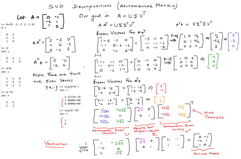
Linear algebra plays a fundamental role in dimensional reduction techniques, which are used to reduce the number of features (dimensions) in a dataset while preserving as much relevant information as possible. Linear algebra techniques like eigen decomposition are commonly used in these methods: Eigenvalue, Eigenvector, Principal Component Analysis (PCA), Singular Value Decomposition (SVD).

Linear Algebra in Feature Engineering

Linear algebra plays a significant role in feature engineering, which is the process of creating new features or transforming existing ones to improve the performance of machine learning models: Feature Transformation, Feature Cross-Products,Feature Selection-Encoding Categorical Variables.

Linear Algebra in Machine Learning Algorithm

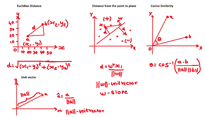
In Mathematics, particularly linear algebra, forms the foundation of many machine learning algorithms: Euclidean Distance, Manhattan Distance, Unit Vector, Distance From point to plane, Kernel function.

Linear Algebra in Recommendation System

Linear algebra plays a fundamental role in recommendation systems, which are algorithms designed to suggest items (e.g., products, movies, music, articles) to users based on their preferences and behavior.for example,Matrix Factorization,User-Item Interaction Matrix,Content-Based Filtering,Collaborative Filtering,Cosine Similarity.

The Bridge Connection: Linear Algebra Empowers Machine Learning

Linear Regression: This fundamental algorithm analyzes relationships between features (independent variables) and a target variable (dependent variable) using a linear model. The model aims to minimize the error between predicted and actual values. Mathematically, the linear model can be represented as:

$$y = w₁x₁ + w₂x₂ + ... + wₙxₙ + b (hypothesis function)$$

where:

• y is the predicted target value

• x₁, x₂, ..., xₙ are the features

• w₁, w₂, ..., wₙ are the coefficients (weights)

Example (Solving Linear Regression with Least Squares):

# Import libraries
import numpy as np

# Sample data (features and target)
X = np.array([[1, 2], [3, 4], [5, 6]])
y = np.array([2, 7, 12])

# Calculate coefficients using least squares (solving linear system)
A = np.concatenate((X, np.ones((X.shape[0], 1))), axis=1)
w = np.linalg.solve(np.dot(A.T, A), np.dot(A.T, y))

# Prediction for a new data point
new_x = np.array([7, 8])
predicted_y = np.dot(w.T, new_x)
print("Predicted value:", predicted_y)

Example (Solving Logistic Regression)

Aim is to code logistic regression for binary classification from scratch, using the raw mathematical knowledge and concept that we have.

First we need to import numpy. NumPy is a class to handle complex array calculation and reduces the time of calculations quickly.

import numpy as np

To package the different methods we need to create a class called “MyLogisticRegression”. The argument taken by the class are:
learning_rate- It determine the learning speed of the model, in gradient descent algorithm
num_iteration- It determine the number of time, we need to run gradient descent algorithm.

class MyLogisticRegression:

    def __init__(self, learning_rate = 1, num_iterations = 2000):
       self.learning_rate = learning_rate
       self.num_iterations = num_iterations
       self.w = []
       self.b = 0

We are all set to go, first the foundation for the main algorithms are to laid.

  def initialize_weight(self,dim):
    """
    This function creates a vector of zeros of shape (dim, 1)      for w and initializes b to 0.
    Argument:
    dim -- size of the w vector we want (or number of parameters  in this case)
    """
       w = np.zeros((dim,1))
       b = 0
       return w, b

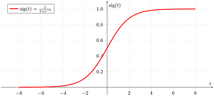
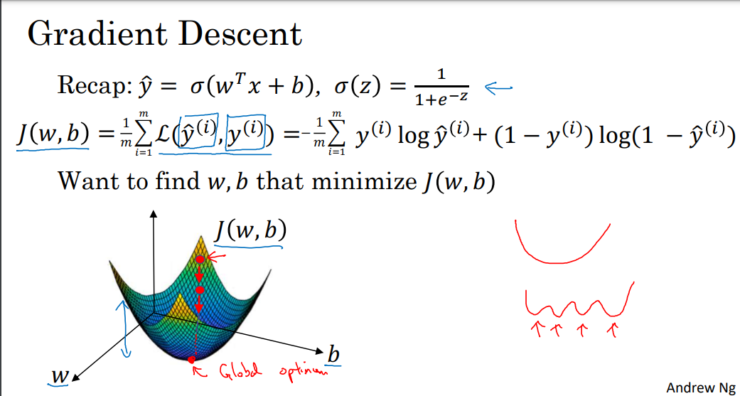
The most basic and essential element of logistic regression is logistic function also called sigmoid.

 def sigmoid(self,z):
    """
    Compute the sigmoid of z
    Argument:
    z -- is the decision boundary of the classifier
    """
        s = 1/(1 + np.exp(-z)) 
        return s

Hypothesis

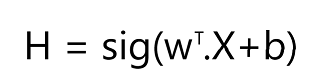
Now we write a function to define the hypothesis. The subscript over ‘w’ stands for transpose of the weight vector.

 def hypothesis(self,w,X,b):
    """
    This function calculates the hypothesis for the present model
    Argument:
     w -- weight vector
     X -- The input vector
     b -- The bias vector
    """
        H = self.sigmoid(np.dot(w.T,X)+b) 
        return H

Cost Function and Gradients

Cost Function is a function that measures the performance of a Machine Learning model for given data. While Gradients quantify, how better the model can perform.

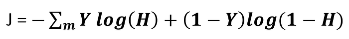
 def cost(self,H,Y,m):
    """
    This function calculates the cost of hypothesis
    Arguments: 
     H -- The hypothesis vector 
     Y -- The output 
     m -- Number training samples
    """
        cost = -np.sum(Y*np.log(H)+ (1-Y)*np.log(1-H))/m 
        cost = np.squeeze(cost)   
        return cost

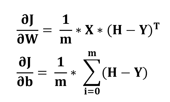
 def cal_gradient(self, w,H,X,Y):
    """
    Calculates gradient of the given model in learning space
    """
        m = X.shape[1]
        dw = np.dot(X,(H-Y).T)/m
        db = np.sum(H-Y)/m
        grads = {"dw": dw,
                 "db": db}
        return grads

    def gradient_position(self, w, b, X, Y):
    """
    It just gets calls various functions to get status of learning model
    Arguments:
     w -- weights, a numpy array of size (no. of features, 1)
     b -- bias, a scalar
     X -- data of size (no. of features, number of examples)
     Y -- true "label" vector (containing 0 or 1 ) of size (1, number of examples)
    """

        m = X.shape[1]
        H = self.hypothesis(w,X,b)         # compute activation
        cost = self.cost(H,Y,m)               # compute cost
        grads = self.cal_gradient(w, H, X, Y) # compute gradient
        return grads, cost

Gradient Descent Algorithm

Gradient descent is an optimization algorithm used to minimize some function by iteratively moving in the direction of steepest descent as defined by the negative of the gradient. In machine learning, we use gradient descent to update the parameters (w ,b ) of our model.

The significance of this algorithm lies in the update rule, which updates the parameters according to their present steepness.

 def gradient_descent(self, w, b, X, Y, print_cost = False):
    """
    This function optimizes w and b by running a gradient descent algorithm

    Arguments:
    w — weights, a numpy array of size (num_px * num_px * 3, 1)
    b — bias, a scalar
    X -- data of size (no. of features, number of examples)
    Y -- true "label" vector (containing 0 or 1 ) of size (1, number of examples)
    print_cost — True to print the loss every 100 steps

    Returns:
    params — dictionary containing the weights w and bias b
    grads — dictionary containing the gradients of the weights and bias with respect to the cost function
    costs — list of all the costs computed during the optimization, this will be used to plot the learning curve.
    """

        costs = []

        for i in range(self.num_iterations):
        # Cost and gradient calculation 
            grads, cost = self.gradient_position(w,b,X,Y)


        # Retrieve derivatives from grads
        dw = grads[“dw”]
        db = grads[“db”]

        # update rule 
        w = w — (self.learning_rate * dw) 
        b = b — (self.learning_rate * db)

        # Record the costs
        if i % 100 == 0:
            costs.append(cost)

        # Print the cost every 100 training iterations
        if print_cost and i % 100 == 0:
             print (“Cost after iteration %i: %f” %(i, cost))


        params = {“w”: w,
                  “b”: b}

       grads = {“dw”: dw,
                “db”: db}

       return params, grads, costs

Predict

Hypothesis function gives us a probability of y = 1. We resolve this by assigning p = 1, for h greater than 0.5.

 def predict(self,X):
    '''
    Predict whether the label is 0 or 1 using learned logistic regression parameters (w, b)

    Arguments:
    w -- weights, a numpy array of size (n, 1)
    b -- bias, a scalar
    X -- data of size (num_px * num_px * 3, number of examples)

    Returns:
    Y_prediction -- a numpy array (vector) containing all predictions (0/1) for the examples in X
    '''
        X = np.array(X)
        m = X.shape[1]

        Y_prediction = np.zeros((1,m))

        w = self.w.reshape(X.shape[0], 1)
        b = self.b
        # Compute vector "H" 
        H = self.hypothesis(w, X, b)

        for i in range(H.shape[1]):
        # Convert probabilities H[0,i] to actual predictions p[0,i]
            if H[0,i] >= 0.5:
                Y_prediction[0,i] = 1
            else: 
                Y_prediction[0,i] = 0

       return Y_prediction

Train Model Function

This method is directly called by the user to train the hypothesis. This is one of the accessible method.

def train_model(self, X_train, Y_train, X_test, Y_test, print_cost = False):
    """
    Builds the logistic regression model by calling the function you’ve implemented previously

    Arguments:
    X_train — training set represented by a numpy array of shape (features, m_train)
    Y_train — training labels represented by a numpy array (vector) of shape (1, m_train)
    X_test — test set represented by a numpy array of shape (features, m_test)
    Y_test — test labels represented by a numpy array (vector) of shape (1, m_test)
    print_cost — Set to true to print the cost every 100 iterations

    Returns:
    d — dictionary containing information about the model.
    """
# initialize parameters with zeros 
        dim = np.shape(X_train)[0]
        w, b = self.initialize_weight(dim)
# Gradient descent 
        parameters, grads, costs = self.gradient_descent(w, b, X_train, Y_train, print_cost = False)

 # Retrieve parameters w and b from dictionary “parameters”
        self.w = parameters[“w”]
        self.b = parameters[“b”]

 # Predict test/train set examples 
        Y_prediction_test = self.predict(X_test)
        Y_prediction_train = self.predict(X_train)
# Print train/test Errors
        train_score = 100 — np.mean(np.abs(Y_prediction_train — Y_train)) * 100
        test_score = 100 — np.mean(np.abs(Y_prediction_test — Y_test)) * 100
        print(“train accuracy: {} %”.format(100 — np.mean(np.abs(Y_prediction_train — Y_train)) * 100))
        print(“test accuracy: {} %”.format(100 — np.mean(np.abs(Y_prediction_test — Y_test)) * 100))
        d = {“costs”: costs,
             “Y_prediction_test”: Y_prediction_test, 
             “Y_prediction_train” : Y_prediction_train, 
             “w” : self.w, 
             “b” : self.b,
             “learning_rate” : self.learning_rate,
             “num_iterations”: self.num_iterations,
             “train accuracy”: train_score,
             “test accuracy” : test_score}

         return d

Testing on a small dataset

#Dataset
X_train = np.array([[5,6,1,3,7,4,10,1,2,0,5,3,1,4],[1,2,0,2,3,3,9,4,4,3,6,5,3,7]])
Y_train = np.array([[0,0,0,0,0,0,0,1,1,1,1,1,1,1]])
X_test  = np.array([[2,3,3,3,2,4],[1,1,0,7,6,5]])
Y_test  = np.array([[0,0,0,1,1,1]])

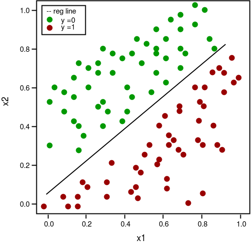
We call the class on default values

clf = MyLogisticRegression()
d = clf.train_model(X_train, Y_train, X_test, Y_test)
print (d["train accuracy"])
#Output
train accuracy: 100.0 %
test accuracy: 100.0 %
100.0

We’ll set a very small learning rate and iteration number

clf = MyLogisticRegression(0.001, 100)
d = clf.train_model(X_train, Y_train, X_test, Y_test)
#Output
train accuracy: 92.85714285714286 %
test accuracy: 83.33333333333334 %

Conclusion: A Journey of Understanding

By understanding the core concepts of linear algebra and their implementation with Python, you gain a deeper appreciation for the inner workings of machine learning algorithms. This knowledge empowers you to troubleshoot, build, and refine your own machine learning models, unlocking their true potential.

Note: This lecture provides a brief overview. Consider including additional details like:

Properties of vectors and matrices (eigenvalues, eigenvectors, etc.)

Solving systems of linear equations with different methods (Gaussian elimination, etc.)

Applications of linear algebra in other machine learning algorithms (dimensionality reduction, etc.)

Bibliography

° Harris CR, Millman KJ, van der Walt SJ, Gommers R, Virtanen P, Cournapeau D, Wieser E, Taylor J, Berg S, Smith NJ, Kern R, Picus M, Hoyer S, van Kerkwijk MH, Brett M, Haldane A, Del Río JF, Wiebe M, Peterson P, Gérard-Marchant P, Sheppard K, Reddy T, Weckesser W, Abbasi H, Gohlke C, Oliphant TE. Array programming with NumPy. Nature. 2020 Sep;585(7825):357-362. doi: 10.1038/s41586-020-2649-2. Epub 2020 Sep 16. PMID: 32939066; PMCID: PMC7759461.

° Choi RY, Coyner AS, Kalpathy-Cramer J, Chiang MF, Campbell JP. Introduction to Machine Learning, Neural Networks, and Deep Learning. Transl Vis Sci Technol. 2020 Feb 27;9(2):14. doi: 10.1167/tvst.9.2.14. PMID: 32704420; PMCID: PMC7347027.

° https://cs229.stanford.edu/lectures-spring2022/main_notes.pdf

° https://see.stanford.edu/materials/aimlcs229/cs229-notes1.pdf